3530
Accelerated Localized Correlated Spectroscopy with Compressed Sensing Reconstruction Using Joint Hankel Low Rank Regularization and Group Sparsity1Radiological Sciences, University of California, Los Angeles, Los Angeles, CA, United States
Synopsis
Compressed sensing (CS) combined with non-uniform undersampling, such as the low-rank Hankel matrix completion method, have accelerated the acquisition time of 2D magnetic resonance spectroscopy (MRS). This technique relies on reconstructing the vector of all t1 points separately for each F2 point. We introduce a CS-based method that implements joint Hankel low rank regularization, which enforces the low-rankness of all Hankel matrices formed from the entire F2-t1 data simultaneously. We compare this method with group sparsity CS reconstruction of retrospectively undersampled localized correlated spectroscopy (COSY) acquisitions in a brain phantom and calf muscle.
Introduction
One-dimensional magnetic resonance spectroscopic (MRS) techniques allow site-specific measurements of metabolite compositions to probe the impact of various pathologies non-invasively. One of the main limitations of 1D techniques is the overlap of spectral peaks. Two-dimensional spectroscopy (2D MRS) can differentiate overlapping peaks but requires an increase in scan time proportional to the number of measured t1 points needed to resolve the additional spectral dimension F11,2. Acceleration methods that combine non-uniform under-sampling (NUS) of t1 with compressed sensing (CS) reconstruction have been proposed to reduce the scan time3,4. CS methods based on group sparsity (GS) have been applied for accelerated 2D correlated spectroscopy (COSY) and shown to outperform maximum entropy and conventional CS reconstruction5,6. Recently, low-rank Hankel matrix completion, which exploits the low rank property of the Hankel matrix formed from all t1 measurements corresponding to any point along F2, has been proposed as an alternative method that can more accurately recover broad peaks compared to l1-norm based CS methods7. This technique relies on reconstructing the vector of all t1 points separately for each F2 point7,8. In this study, we introduce a CS-based method that implements joint Hankel low rank (JHLR) regularization, which enforces the Hankel low-rankness of all matrices formed from the entire F2-t1 data simultaneously. We compare this method with GS reconstruction of retrospectively undersampled brain phantom and calf-muscle localized correlated spectroscopy (L-COSY) acquisitions.Methods
The reconstruction of the F2-t1 data x using JHLR regularization is posed as the following minimization problem: $$\operatorname*{min}_{x \in \mathbb{C}^{N_{2} \times N_{1}}} \frac{1}{2}\| y - Ax\|^{2}_{2} + \tau \sum_{n = 1}^{N_2} \|H_{n} x\|_{S_{1}}$$ where y is the under-sampled F2-t1 data, A is the undersampling operator, N1 the number of F1 points, N2 the number of F2 points,$$$\| \cdot \|_{S_{1}} $$$ denotes the Schatten 1-norm9 , $$$ \tau $$$ is a regularization parameter, and Hn is the operator that forms a Hankel matrix from all t1 measurements corresponding to the nth F2 point of x. The regularization parameters for each algorithm were chosen empirically as those minimizing the normalized root mean square error (nRMSE) for selected diagonal and cross peaks. Both the JHLR and GS algorithms are based on the alternating direction method of multipliers (ADMM)10,11
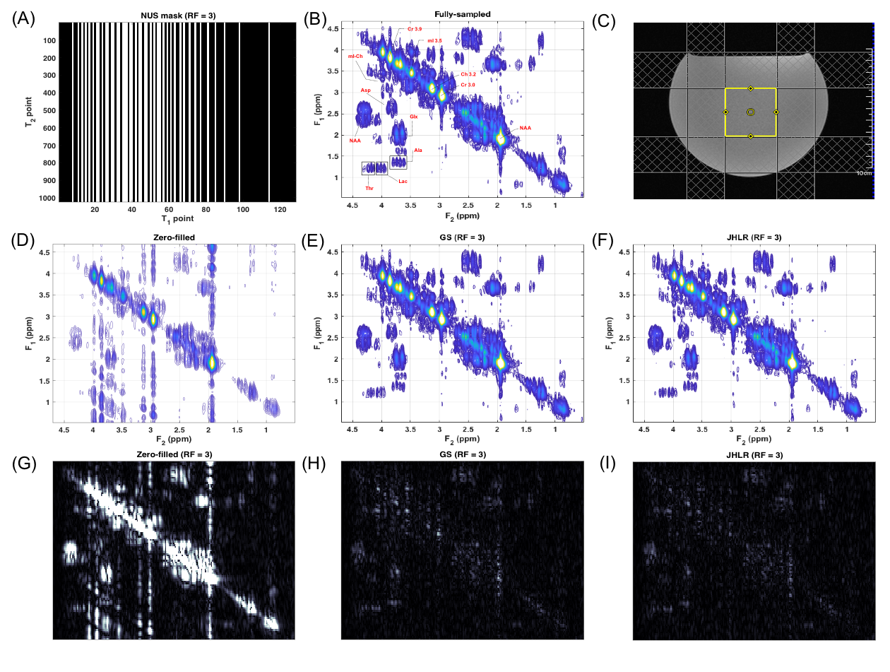
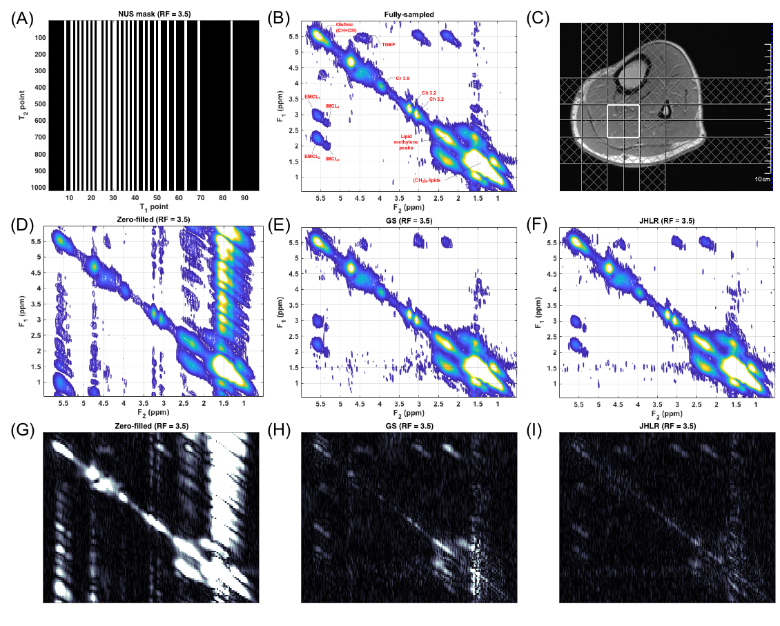
A COSY spectrum of a brain phantom composed of several metabolites at physiological concentrations was acquired with the following parameters: VOI = 3x3x3 cm3, TR=2 s, TE=30 ms, 1024 t2 points, 128 t1 points, BW2=2000 Hz, BW1=1250 Hz, and 12 averages. A COSY spectrum of the soleus calf muscle from a healthy volunteer was acquired with: VOI = 2.5x2.5x2.5 cm3, TR=1.5 s, TE=30 ms, 1024 t2 points, 96 t1 points, BW2=2000 Hz, BW1=1250 Hz, and 8 averages. These data sets were retrospectively undersampled at reduction factors (RF) of 2, 2.5, 3, 3.5, 4, and 5 using NUS masks generated with a skewed sine bell squared sampling density function.
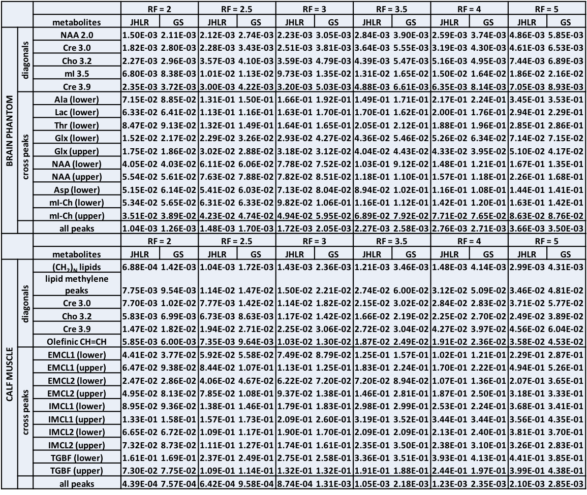
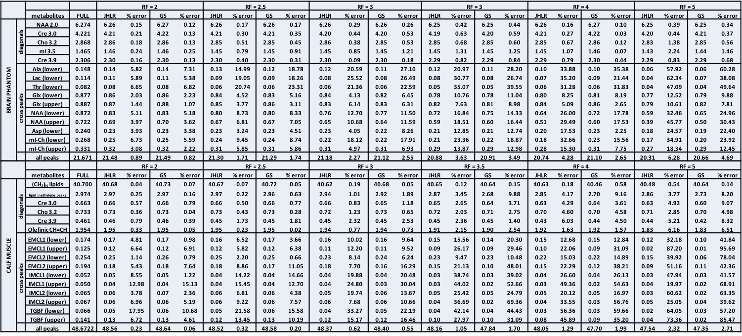
To assess reconstruction and quantitation accuracy, the peak integrals of the fully-sampled, GS-reconstructed, and JHLR-reconstructed spectra were computed, as well and the nRMSE’s of selected diagonal and cross peaks. For the brain phantom the diagonal peaks are: N-acetylaspartate (NAA), Creatine (Cr-3.0), Choline (Ch-3.2), myo-Inositol (mI-3.2), and Cr-3.9; the cross peaks are: Alanine (Ala), Lactate (Lac), Threonine (Thr), glutamine/glutamate (Glx), N-acetylaspartate (NAA), Aspartate (Asp), and mI-Ch. For the calf muscle, the diagonal peaks are the (CH2)N lipids, lipid methylene peaks, Cr-3.0, Ch-3.2, Cr-3.9, and the olefinic (CH=CH) peaks; the cross peaks are the extra- and intra-myocellular lipids (EMCL1/EMCL2 and IMCL1/IMCL2) and the triglyceride backbone fatty (TGBF) acids.
Results
In almost all cases, Table 2 shows that JHLR produces lower percent errors of the peak integrals compared to GS. Similarly, Table 1 shows that JHLR generally gives lower nRMSE values for most peaks at all reduction factors. Figures 1 and 2 demonstrate the comparable performance of GS and JHLR in reconstructing the calf and brain COSY spectra, although the difference maps indicate that JHLR recovers the spectra with higher reconstruction accuracy.Discussion
Both JHLR and GS perform comparably in reconstructing the retrospectively undersampled brain phantom and calf muscle data. However, as seen by the absolute difference maps, peak integrals, and nRMSE values, JHLR results in the most accurate COSY reconstructions. Results indicate that this method is a competitive alternative to existing reconstruction techniques for accelerated localized 2D MRS.Conclusion
This study has introduced a novel low-rank based regularization technique for accelerated 2D MRS. Compared with group sparsity-based CS reconstruction, JHLR regularization has shown greater accuracy quantitatively both in terms of peak integrals and nRMSE’s of reconstructed peaks. Future work includes extending JHLR-based CS reconstruction to multi-dimensional 2D spectroscopic imaging.Acknowledgements
Grant support NIH/NIBIB - 5R21EB020883-02References
[1] Thomas, M.A., et al. Localized two-dimensional shift correlated MR spectroscopy of human brain. Magnetic Resonance in Medicine, 2001; 46(1): 58-67.
[2] Thomas, M.A., et al. Evaluation of two-dimensional L-COSY and JPRESS using a 3T MRI scanner: from phantoms to human brain in vivo. NMR in Biomedicine, 2003; 16(5):245-251.
[3] Furuyama, J.K., et al. Application of Compressed Sensing to Multi-dimensional Spectroscopic Imaging in human prostate. Magnetic Resonance in Medicine, 2012; 67(6):1499-1505.
[4] Wilson, N.E., et al. Accelerated Five-dimensional Echo Planar J-resolved Spectroscopic Imaging: Implementation and pilot validation in human brain. Magnetic Resonance in Medicine, 2016; 75(1):42-51.
[5] Burns, B.L., et al. Group Sparse Reconstruction of Multi-dimensional Spectroscopic Imaging in Human Brain in vivo. Algorithms, 2014; 7(3):276-294.
[6] Burns, B.L., et al. Non-Uniformly under-sampled Multi-dimensional Spectroscopic Imaging in vivo: maximum entropy versus compressed sensing reconstruction. NMR in Biomedicine, 2014; 27(2):191-201.
[7] Qu, X., et al. Accelerated NMR Spectroscopy with Low-Rank Reconstruction. Angewandte Chemie International Edition, 2015; 54(3):852-854.
[8] Guo, D., et al. A Fast Low Rank Hankel Matrix Factorization Reconstruction Method for Non-Uniformly Sampled Magnetic Resonance Spectroscopy. IEEE Access, 2017; 5:16033-16039.
[9] Lefkimmiatis, S., et al. Hessian Schatten-norm Regularization for Linear Inverse Problems. IEEE Transactions on Image Processing, 2013; 22(5):1873-1888.
[10] Goldstein, T., Osher, S. The Split-Bregman Method for L1-regularized problems. SIAM Journal on Imaging Sciences, 2009; 2(2):323-343.
[11] Afonso, M.V., et al. An Augmented Lagrangian Approach to the Constrained Optimization Formulation of Imaging Inverse Problems. IEEE Transactions on Image Processing, 2011; 20(3):681-695.
Figures