3513
Whole-Volume, High-Resolution, In-Vivo Signal-to-Noise Ratio and G-factor Superiority, and Structural Similarity Index Differences, of Compressed Sensing SPACE and CAIPIRINHA SPACE over GRAPPA SPACE1Radiology, Johns Hopkins Hospital, Baltimore, MD, United States, 2Microsoft Corporation, Redmond, WA, United States, 3Johns Hopkins Hospital, Baltimore, MD, United States
Synopsis
Compressed Sensing, CAIPIRINHA, and GRAPPA techniques reduce MRI acquisition times. We used a 3-dimensional sliding region-of-interest analysis tool to perform parameter-controlled, whole-volume average signal-to-noise ratio and g-factor comparison, and g-factor structural similarity index measurements (SSIM) of the above techniques in the setting of 3 Tesla knee MRI. We demonstrate g-factor superiority of CS SPACE over CAIPIRINHA SPACE and g-factor superiority of CAIPIRINHA SPACE over GRAPPA SPACE in living subjects. Post-processing, including pre-scan normalize and distortion correction, improves g-factors and causes variation in the g-factor SSIM results between the techniques.
Introduction
Parallel imaging techniques, such as GRAPPA and CAIPIRINHA, exploit differential coil spatial sensitivities1, and Compressed Sensing (CS) capitalizes on wavelet transform domain sparsity to reduce acquisition times.2,3 Elucidating the parameter-controlled, whole-volume signal-to-noise ratio (SNR) and geometry (g) factor performance of these techniques is important for understanding potential trade-offs in musculoskeletal MRI. Additionally, application of whole-volume structural similarity index measurements (SSIM)4 to SNR and g-factor for structural similarity comparison between the techniques has not been previously demonstrated.Purpose
To determine in living subjects whether 3D CS SPACE TSE, 3D CAIPIRINHA SPACE TSE, or 3D GRAPPA SPACE TSE produces the best whole-volume average SNR and geometry (g) factor, determine the g-factor SSIM between techniques, and determine the effects of post-processing, including pre-scan normalize and distortion correction, on g-factor performance of the techniques for knee MRI.Materials and Methods
SNR and G-factor Calculation
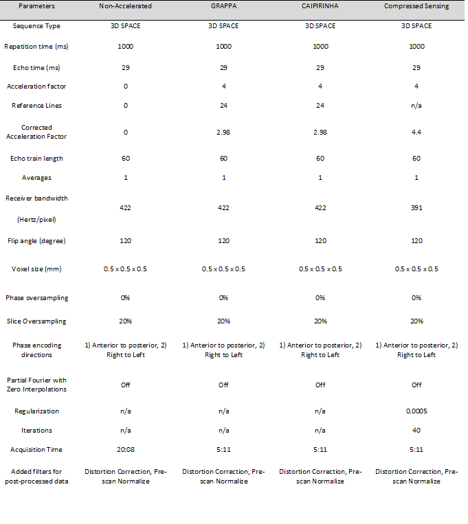
Whole-volume average SNR and g-factor of 4-fold CS-, CAIPIRINHA- and GRAPPA-accelerated 3D SPACE TSE were assessed in 12 knees on 3 Tesla MRI. A previously validated 3-dimensional whole-volume SNR and g-factor sliding region-of-interest (ROI) analysis tool that uses the difference method5-8 was used for evaluation. The following formulas were utilized;
SNR = [average (SROI1, SROI2)]/[√2 *standard deviation(SROI1-SROI2)], where SROI represents the average signal on each matching ROI on two repeat images6, and;
G factor = [SNRun-accelerated/(SNRaccelerated * √R)], where R = acceleration factor6.
We used 1 cm3 contiguous ROIs to maintain spatial resolution while minimizing local noise variability, motion effects and divide-by-zero g-factor errors. Planar averages were used as the index units of analysis for computational simplicity. R values were corrected by number of auto-calibrating reference lines7. The corrected “acceleration” factor of CS was determined by the k-space sampling factor. CS whole volume average SNR was corrected for receiver bandwidth differences (Figure 1) by a factor of 1/√(422/391).
SSIM Calculation
Pairwise g-factor SSIM between techniques were calculated. The following formula was utilized;
SSIM = (2μxμy+C1)(2σxy+C2) ∕ (μx2+μy2+C1)( σx2+ σy2+C2); where μ = ROI average, σ = ROI standard deviation and σxy= (1/N-1) ∑ (xi-μx)(yi-μy) where i is the ith voxel in the ROI, 1<i<N.4 In accordance with Wang4, k1=0.1 and k2=0.3, where C1 = k1*pixel range and C2 = k2*pixel range.
Outcome color maps were created using unit scaled values for the Hue variable in the HSV color scheme.
Statistics
Paired-samples-T and one-factor-ANOVA tests were used to evaluate differences between techniques, pre- and post-processed data, accelerated and non-accelerated axes, and patients. P-values < 0.01 were considered significant.
Results
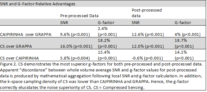
For post-processed data, CS demonstrated a 12% SNR and 18.7% g-factor advantage over GRAPPA (p<0.001 for both), and CAIPIRINHA demonstrated a 12.6% SNR and 4% g-factor advantage over GRAPPA (p<0.001 for both) (Figures 2 and 3). For pre-processed data, CS demonstrated a 16% SNR and 18.2% g-factor advantage over GRAPPA (p<0.001 for both), and CAIPIRINHA demonstrated a 9.6% SNR and 2.4% g-factor advantage over GRAPPA (p<0.001 for both) (Figure 2). Apparent “discordance” between average SNR and g-factor values is produced by mathematical aggregation following local SNR and g-factor calculation. Post-processed data aggregated across all techniques demonstrated superior g-factors compared to pre-processed data (5.7%, p<0.001).
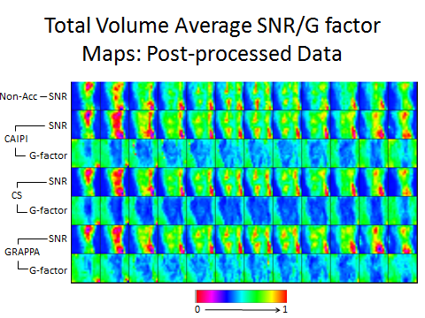
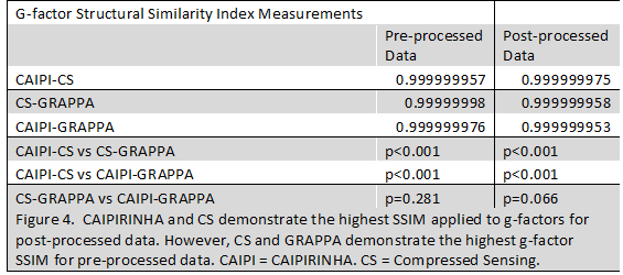
Average whole-volume SNR and G-factor SSIM results are shown in Figure 4. Figure 5 displays corresponding SNR and g-factor SSIM color maps for post-processed data. All pair-wise comparisons demonstrated very high SSIMs. While CAIPIRINHA and CS demonstrated the highest post-processed data SSIM, CS and GRAPPA demonstrated the highest pre-processed data SSIM (p<0.001 for both).
Between subject g-factor differences for post-processed data served as a negative control and were not significantly different (p = 0.977). G-factor variance across accelerated and non-accelerated imaging axes served as a positive control (7) and the non-accelerated axis g-factor variance was 578% and 274% more than the accelerated axes, p<0.001 for both).
Conclusion
We demonstrate the whole-volume average g-factor superiority of 3D CS SPACE TSE over 3D CAIPIRINHA SPACE TSE, and 3D CAIPIRINHA SPACE TSE over 3D GRAPPA SPACE TSE in the knee in living subjects. Post-processing improved whole volume average g-factors and caused variation in the g-factor SSIM results between the techniques. Practically, the immediate utility of CAIPIRINHA is suggested given the post-procedural computational burden of CS. The improvement of CAIPIRINHA in whole-volume average SNR by ~12.6% compared to GRAPPA, in combination with decreased intrinsic aliasing, indicates increased suitability for musculoskeletal evaluations.Acknowledgements
No acknowledgement found.References
1. Breuer FA, Blaimer M, Heidemann RM, Mueller MF, Griswold MA, Jakob PM. Controlled aliasing in parallel imaging results in higher acceleration (CAIPIRINHA) for multi-slice imaging. Magn Reson Med. 2005 Mar;53(3):684-91.
2. Michael Lustig, David Donoho, and John M. Pauly. Sparse MRI: The Application of Compressed Sensing for Rapid MR Imaging. Magnetic Resonance in Medicine 58:1182–1195 (2007).
3. Fritz J, Ahlawat S, Demehri S, Thawait GK, Raithel E, Gilson WD, Nittka M. Compressed Sensing SEMAC: 8-fold Accelerated High Resolution Metal Artifact Reduction MRI of Cobalt-Chromium Knee Arthroplasty Implants. Invest Radiol. 2016 Oct;51(10):666-76.
4. Image Quality Assessment: From Error Visibility to Structural Similarity. Zhou Wang, Alan Conrad Bovik, Hamid Rahim Sheikh, and Eero P. Simoncelli. Ieee transactions on image processing, vol. 13, no. 4, april 2004.
5. M J Firbank, A Coulthard, R M Harrison, Williams ED. A comparison of two methods for measuring the signal to noise ratio on MR image. Phys. Med. Biol. 44 (1999) N261–N264.
6. S. B. Reeder, B. J. Wintersperger, O. Dietrich, T. Lanz, A. Greiser, M. F. Reiser, G. M. Glazer, and S. O. Schoenberg, “Practical approaches to the evaluation of signal-to-noise ratio performance with parallel imaging: Application with cardiac imaging and a 32-channel cardiac coil,” Magn. Reson. Med. 54, 748–754 (2005).
7. F. L. Goerner and G. D. Clarke: Signal-to-noise ratio in parallel imaging MRI. Medical Physics, Vol. 38, No. 9, September 2011.
8. Gizewski ER, Maderwald S, Wanke I, Goehde S, Forsting M, Ladd ME (2005) Comparison of volume, four- and eightchannel head coils using standard and parallel imaging. Eur Radiol 15:1555–1562.
Figures