3506
Parameter Optimization of Wave-CAIPI Based on Theoretical Analysis1Paul C. Lauterbur Research Center for Biomedical Imaging, Shenzhen Institutes of Advanced Technology, Chinese Academy of Sciences, Shenzhen, China, 2Department of Biomedical Engineering and Department of Electrical Engineering, University at Buffalo, The State University of New York, Buffalo, NY, United States
Synopsis
Wave-CAIPI is an novel 3D imaging technique with corkscrew trajectory in k-space to reduce g-factor penalty and speed up MRI acquisitions. The sinusoidal gradient parameters of Wave-CAIPI, amplitude and cycles, play an important role since they determine the point spread function of the trajectory and thus the final reconstruction. However, how to choose the optimal sinusoidal gradient parameters which leads to the minimal g-factor has not been exploited. In this work, we theoretically analyzed the influence of the sinusoidal gradient parameters on g-factor. An optimization algorithm which can be automatically conducted is then proposed to optimize these parameters for achieving minimal g-factor penalty. The simulations show that using the optimized sinusoidal gradient parameters can achieve lower g-factor penalty in Wave-CAIPI reconstructions.
Introduction
In practical parallel imaging, acceleration factor is ultimately limited by spatially noise amplification, which is characterized by g-factor. Recently, Wave-CAIPI1 was proposed for 3D imaging to significantly reduce the g-factor by playing sinusoidal gradients during the readout time, leading to corkscrew trajectory in k-space. The sinusoidal gradient parameters of Wave-CAIPI, amplitude and cycles, play an important role since they determine the point spread function (PSF) of the trajectory and thus the final reconstruction2. However, how to choose the optimal parameters which leads to minimal g-factor has not been exploited. In this work, the influence of the parameters of the sinusoidal gradients on the g-factor penalty in Wave-CAIPI was theoretically analyzed. And then, an optimization scheme is proposed to guide choosing the sinusoidal gradient parameters of Wave-CAIPI.
Theory and Methods
Wave-CAIPI can be viewed as a generalized SENSE3 model: $$$wave[x,y,z]=Em[x,y,z]$$$ and the g-factor can be generalized as:
$$g_\rho=\sqrt{(E^{H}E)_{\rho,\rho}^{-1}(S^{H}S)_{\rho,\rho}}$$
where $$$E=MF_x^{-1}Psf[k,y,z]F_xC$$$, and $$$C$$$ is the sensitivity encoding matrix in Wave-CAIPI, $$$S$$$ the sensitivity encoding matrix in SENSE3, $$$M$$$ the aliasing matrix due to undersampling, and $$$Psf[k,y,z]$$$ the PSF caused by sinusoidal gradients during readout. Since the g-factors of Wave-CAIPI reconstruction distribute homogeneously, the mean g-factor can be calculated and simplified by:
$$g_{mean}=\frac{1}{N_\rho}\sum_{\rho=1}^{N_\rho}g_{\rho}\approx g_c+\eta(g_c-1)$$
where $$$N_\rho$$$ is the number of voxels in the ROI, $$$g_c$$$ is the g-factor in the central voxel. $$$\eta(g_c-1)$$$ is the first order correction term describing the discrepancy between $$$g_{mean}$$$ and $$$g_c$$$. The coefficient $$$\eta$$$ (at the range of $$$[-1,0]$$$) is estimated by a few g-factor maps calculated using the pseudo multiple approach4.
Let $$$g_{mean}(a,c)$$$ denotes a map showing g-factors over relative amplitude $$$a$$$ ($$$amplitude=a\cdot G_x$$$) and cycles ($$$c$$$), which can be calculated theoretically as mentioned above or using pseudo multiple replica (Fig 1).
Concretely,
$$Psf[k,y,z]=e^{-i2\pi(P_y[k]y+P_z[k]z)}$$
$$=e^{-i \frac{a}{c} \triangle k_xN_x [(1-cos(2\pi c \frac{k}{N_x}))y+sin(2\pi c \frac{k}{N_x})z]}$$
Obviously, there is a periodic relationship between $$$a$$$ and $$$Psf[k,y,z]$$$ but the periods are different with different values of $$$k$$$, $$$y$$$ and $$$z$$$ (Fig 2a). Therefore, g-factor exhibits an approximate periodicity over the amplitude of sinusoidal gradients (Fig 1). On the contrary, $$$Psf[k,y,z]$$$ shows irregular oscillation along the cycle ($$$c$$$) direction when $$$c$$$ is small and tends to be stable when $$$c$$$ is large (Fig 2b). Therefore, g-factor is showing little and almost no regular change along the cycle direction (Fig 1).
We prefer a local parameter optimization rather than global parameter optimization for the following reasons:
- $$$g_{mean}(a,c)$$$ map as seen in Fig. 1. is not a convex function but with many stationary points;
- The amplitude and slew rate of the sinusoidal gradients are limited due to engineering and physiological constraints;
- $$$g_{mean}(a,c)$$$ map is showing little change along the cycle direction and there's no need to optimize the parameter $$$c$$$.
Therefore, we propose a local optimization method using gradient descent in this work. Concretely, the amplitude $$$a$$$ is updated by,
$$a^{new}=a+\triangle a=a-\alpha \frac{\partial g_{mean}(a,c)}{\partial a}$$
where
$$\frac{\partial g_{mean} (a,c)}{\partial a}=\frac{1}{N_\rho}\sum_{\rho=1}^{N_\rho}\frac{\partial g_\rho}{\partial a}=(1+\eta)\frac{\partial g_c}{\partial a}$$
and
$$\frac{\partial g_c}{\partial a}=\frac{-\sqrt{(S^HS)_{c,c}}}{\sqrt{(E^HE)_{c,c}^{-1}}}Re\{[(E^HE)^{-1}(E^H\frac{\partial E}{\partial a})(E^HE)^{-1}]_{c,c}\}$$
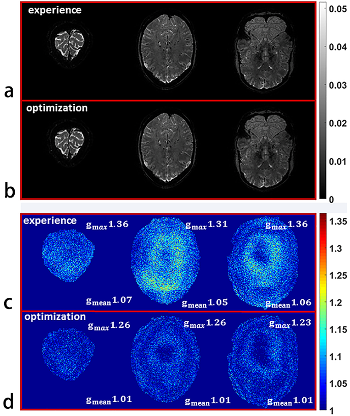
A 3D Wave-CAIPI data were acquired by Bilgic B. et. al.1 with the following parameters: $$$FOV=240 \times 240 \times 120 mm^3$$$; $$$1 mm^3$$$ isotropic voxel size; $$$TR=40ms$$$; $$$bandwidth=70 Hz/pixel$$$; six-fold oversampling; 32 receive coils. Simulations and reconstructions with acceleration of $$$R_y\times R_z=3\times 3$$$ were performed. The g-factor maps were calculated by using pseudo multiple replica approach4. With different amplitudes ($$$a\cdot G_x$$$) and cycles ($$$c$$$), the $$$g_{mean}(a,c)$$$ map was obtained.
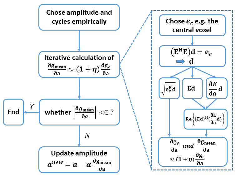
Additionally, for mutual verification, the theoretical $$$g_{mean}(a,c)$$$ was also calculated (Fig 1), with $$$\eta=-0.5$$$. The flowchart of the proposed local optimization scheme is shown in Fig 3, where the details of the second step are described in the dotted box and the inner step in calculating $$$\frac{\partial g_c}{\partial a}$$$ is solved with MATLAB's LSQR function.
Results
Fig 1a and Fig 1b show the $$$g_{mean}(a,c)$$$ calculated by using the pseudo multiple replica approach4 and Fig 1c and Fig 1d show the theoretically calculated $$$g_{mean}(a,c)$$$. One-dimensional views with $$$cycle=7$$$ (Fig 1e) and $$$cycle=9$$$ (Fig 1f) are shown for comparision. These two maps are highly consistent. Using the proposed method, an instance was performed, showing that the maximum g-factor and the mean g-factor with optimized parameters (Fig 4d) are lower than that with the empirically chosen parameters (Fig 4c).
Conclusion and Discussion
In this work, the influence of the amplitude and cycles of sinusoidal gradients on the g-factor of Wave-CAIPI reconstruction is theoretically analyzed. The proposed automatic optimization approach can achieve lower g-factor and be used as a guideline of choosing parameters in Wave-CAIPI. The theoretical analysis of the g-factor in this work is invalid in nonlinear reconstruction like CS-Wave5. Otherwise, the gradient waveforms might be optimized to further achieve lower g-factor in Wave-CAIPI which is out of scope of this paper.
Acknowledgements
The authors thank Dr. Berkin Bilgic for making available the Wave-CAIPI MATLAB code at http://martinos.org/~berkin/software.html. This work is supported in part by the National Natural Science Foundation of China (61471350) and the Science and Technology Program of Guangdong (2015A020214019).
References
1. Bilgic B, Gagoski BA, Cauley SF, Fan AP, Polimeni JR, Grant PE, Wald LL, Setsompop K. Wave-CAIPI for highly accelerated 3D imaging. Magn. Reson. Med. 2015;73(6):2152-2162.
2. Cauley S. F., Setsompop, K., Bilgic, B., Bhat, H., Gagoski, B. and Wald, L. L. Autocalibrated wave-CAIPI reconstruction; Joint optimization of k-space trajectory and parallel imaging reconstruction. Magn. Reson. Med. 2017;78(3):1093-1099.
3. Prussmann KP, Weiger M, Scheidegger MB, Boesiger P. SENSE:sensitivity encoding for fast MRI. Magn. Reson. Med. 1999;42;952-962.
4. Robson PM, Grant AK, Madhuranthakam AJ, Lattanzi R, Sodickson DK, Mckenzie CA. Comprehensive Quantification of SNR Ratio and g-Factor for Image-Based and k-space Based Parallel Imaging Reconstructions. Magn. Reson. Med. 2008;60(4):895-907.
5. Curtis A, Bilgic B, Setsompop K, Menon R, Anand C. Wave-CS: Combining wave encoding and compressed sensing. In: Proc. Intl. Soc. Mag. Reson. Med. 23. ; 2015. p. 82.
Figures
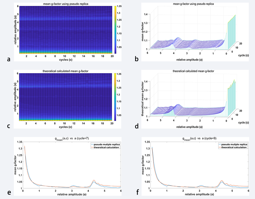
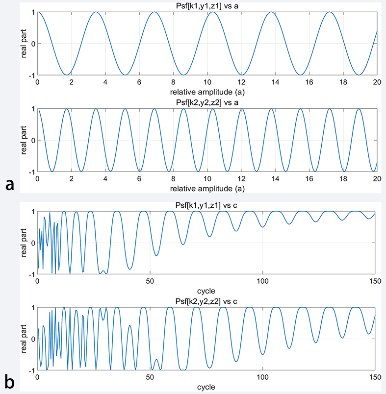
Fig. 2. There is a periodic relationship between the amplitude ($$$=a\cdot G_x$$$) and $$$Psf[k,y,z]$$$ but the periods are different with different $$$k$$$, $$$y$$$ and $$$z$$$ such as $$$(k_1,y_1,z_1)=(100,120,0)$$$ and $$$(k_2,y_2,z_2)=(100,123,0)$$$ (a). On the contrary, $$$Psf[k,y,z]$$$ shows irregular oscillation along the cycle ($$$c$$$) direction when $$$c$$$ is small and tends to be stable when $$$c$$$ is large.