3504
Analysis of longitudinal MRI changes using mixed effects models on deformation tensors1University of Wisconsin Madison, Madison, WI, United States, 2University of Utah, Salt Lake City, UT, United States, 3Harvard Medical School, Cambridge, MA, United States, 4Brigham Young University, Provo, UT, United States
Synopsis
Mixed effects models that include fixed and factor-specific (also known as random) effects offer a natural framework for studying longitudinal MRI data. This work extends mixed effects models to the setting where the responses lie on curved spaces such as the manifold of symmetric positive definite matrices. By treating the subject-wise diffeomorphic deformations between consecutive time points as a field of Cauchy deformation tensors, our framework can facilitate longitudinal analysis that respects the geometry of such data. While the existing body of work dealing with regression models on manifold-valued data is inherently restricted to cross-sectional studies, the proposed mixed effects formulation significantly expands the operating range of longitudinal analyses.
Introduction
Diffeomorphic transformations between longitudinal MRI images could offer unique insight into imaging biomarker progression in development, aging and disease progression. The Cauchy deformation tensors derived from these transformations are highly structured data and lie in the space of symmetric positive definite $$$(\mathtt{SPD})$$$ matrices. It has been widely accepted that the statistical and machine learning models are much more effective if they are endowed with the knowledge of geometry of the data space1. However majority of the models that respect data space geometry have been non-parametric with only recent emerging interest in parametric models. Parametric models have unique advantages of interpretability especially in the clinical/biomedical imaging setting. One such family of models is the so-called mixed effects models2,3 which have extensive applicability for longitudinal data analysis (Fig.1). Surprisingly, very few methods exist for estimating mixed effects models on manifold-valued structured data. Only recently a result on mixed effects models was presented4 that deals with univariate manifold $$$[0,1]$$$, which is the unit interval on a real line $$$\mathbf{R}$$$ with a specifically designed metric to capture sigmoid function like patterns. This work does not deal with the $$$\mathtt{SPD}(3)$$$ manifold and it is computationally impractical for more than a few hundred voxels. This work extends the operating range of mixed effects models for manifold-valued data beyond univariate manifolds. Specifically, formulation for the $$$\mathtt{SPD}(3)$$$ manifold were derived and efficient estimation schemes were developed which significantly expand the range of applicability of the models to large datasets (e.g. estimating these models in over a 100 thousand voxels of brain).Methods
Data. $$$T_1$$$-weighted MRI data from a group of $$$n=185$$$ (109 autistic and 76 control) individuals in the age range of 3 to 52 years were used in the empirical analysis. The individuals were scanned up-to $$$T=4$$$ different time points giving a total of $$$504(<nT=740)$$$ images. These data were processed respecting the longitudinal nature of the data. The longitudinal diffeomorphic changes between consecutive time points were parallel transported5 along the cross-sectional (also diffeomorphic) transformations to a standardized coordinate system (template), thus enabling voxelwise mixed model analysis while reducing the confounding effect of cross-sectional (inter-subject) changes on the longitudinal (intra-subject) changes. The gradient tensor of these longitudinal spatial deformations, $$$F$$$ relates the volumes of voxels between consecutive time points as $$$dv_{t+1}=\mathtt{det}(F)dv_{t}$$$. While $$$\mathtt{det}(F)$$$ captures volumetric changes, it remains invariant to early volume-preserving geometric changes that could potentially be biologically relevant later on. Having the ability to monitor such changes could enable early detection of disease processes and improve the temporal resolution at which the longitudinal effects can be detected. This could be achieved by applying the mixed models directly on the right Cauchy deformation tensor $$$\sqrt{F^TF}$$$. Models. For simplicity the ideas are presented in the Euclidean setting using one factor $$$(\beta_1)$$$ and an offset $$$(\beta_0)$$$. In a fixed effects model one parameter $$$(\beta)$$$ is estimated per factor of interest ($$$x$$$) influencing the out come variable ($$$y$$$), for the whole sample. If we have $$$n$$$ samples, a fixed model solves the following set of equations $$\{y_i=\beta_0+\beta_1x_i\}_{i=1}^n.$$ If there were data from $$$T$$$ time points then the same model would solve the set $$\{\{y_{it}=\beta_0+\beta_1x_{it}\}_{i=1}^n\}_{t=1}^T.$$ Now since each subject is repeated $T$ times it would be natural to include a subject specific offset. Then the set of equations would be $$\{\{y_{it}=\beta_0+\beta_1x_{it}+\beta_{01}\delta_{i1}+\beta_{02}\delta_{i2}+\cdots+\beta_{0n}\delta_{in}\}_{i=1}^n\}_{t=1}^T,$$ where $$$\delta_{ij}$$$ is the Kronecker delta. In linear algebraic form and generalizing to $$$p$$$ fixed covariates these equations would be represented as, $$\mathbf{Y}^{nT\times 1}=\mathbf{X}^{nT\times 1}\mathbf{\beta}^{(p+1)\times 1}+\mathbf{\delta}^{nT\times n}\mathbf{\beta_{0}}^{n\times 1}.$$ The result from solving this linear algebraic equation would estimate a commonly used mixed model with subject-specific intercepts. The commonly used mixed model can be made richer by subject-specific slopes. An equation then would be $$y_{it}=\beta_0+\beta_1\left(\alpha_i\left(x_{it}-\tau_i-t_0\right)-t_0\right)+\beta_0\delta\textrm{-terms}.$$ Note that while $$$\beta$$$, the group specific slope is $$$\frac{\partial y}{\partial x}$$$, $$$\alpha_i=\frac{\partial_t y_i}{\partial_t x_i},$$$ represents subject specific "acceleration'' with an interpretation that $$$\alpha_i<\beta_1$$$ means the sample $$$i$$$ has slower progression compared to the group and vice versa. $$$\tau_i$$$ represents subject-specific shift in onset time with $$$(>0)$$$ indicating late onset and vice versa (Fig.1). While for simplicity the ideas were presented assuming flat Euclidean space, the algorithms were developed for estimating these using the $$$\mathtt{Exp}$$$, $$$\mathtt{Log}$$$ and parallel transport (Fig.2) on the $$$\mathtt{SPD}(3)$$$ manifold and computationally practical heuristics.Results
Representative results from estimating the following mixed models are presented in Figs.3,4,5, $$\mathtt{CDT}=\beta_0+\beta_1\left(\alpha_i(\textrm{age}-\tau_i-t_0)-t_0\right),$$ $$\mathtt{CDT}=\beta_0+\beta_1\left(\alpha_i(\textrm{verbal_iq}-\tau_i-t_0)-t_0\right),~\textrm{and}$$ $$\mathtt{CDT}=\beta_0+\beta_1\left(\alpha_i(\textrm{social_responsiveness_scale}-\tau_i-t_0)-t_0\right).$$
Fig.3 visualizes the estimated $$$\alpha$$$s,$$$\tau$$$s. Fig.4 shows contours of the cumulative link model, $$$\textrm{logit}\left(p\left(\textrm{ADOS}<\textrm{discrete-level}\right)\right)=\beta_0+\beta_1\alpha+\beta_2\tau$$$. Fig.5 shows the scatter of subjects on the $$$\alpha,\tau$$$ axes.
Discussion and conclusions
Methods for performing longitudinal MRI analysis using mixed effects models on the manifold of Cauchy deformation tensors including representative set of empirical results (subset of a more comprehensive set) on an autism study were presented.Acknowledgements
NIH grants R01-EB022883, U54-HD090256 and R01-MH080826 and support from several team members are gratefully acknowledged.References
1. Srivastava, A, Turaga, P, et al. Riemannian Computing in Computer Vision. Springer, 2016.
2. Lindstrom, M, Bates, D. Newton-Raphson and EM algorithms for linear mixed-effects models for repeated-measures data. Journal of the American Statistical Association. 1988; 83(404):1014-1022.
3. Lindstrom, M, Bates, D. Nonlinear mixed effects models for repeated measures data. Biometrics. 1990;673-687.
4. J.-B. Schiratti, J.-B, Allassonniere, S, et al. Learning spatiotem-poral trajectories from manifold-valued longitudinal data. Neural Information Processing Systems (NIPS). 2015; 2404-2412.
5. Lorenzi M, Pennec X. Efficient parallel transport of deformations in time series of images: from Schild's to pole ladder. Journal of Mathematical Imaging and Vision. 2014; 50(1-2):5-17.
6. Turner A, Greenspan K, van Erp T. Pallidum and lateral ventricle volume enlargement in autism spectrum disorder. 2016;252:40-45.
Figures

The key effects for performing analysis of longitudinal changes in MRI. Left: Each subject could have a different progression rate (acceleration effect) of brain atrophy and a different onset for atrophy (time shift effect). A general linear model (GLM) with only fixed effects is insufficient to capture such effects. A mixed effects model including subject-specific (or factor-specific more generally) slope and intercept captures the effects. Right: A simulated data setting demonstrating that our core computational algorithms can be used in estimating these effects when using the entire longitudinal deformation tensor rather than just its determinant. High resolution image available online.
Conceptually core components needed in estimating the acceleration and time shift effects (c.f. Fig. 1) on the deformation manifolds. The exponential ($$$\mathtt{Exp}$$$) and logarithm ($$$\mathtt{Log}$$$) operators (left) and parallel transport of tangent vectors along geodesics (right) on a unit sphere (2-dimensional manifold). These three operators provide the framework for estimating distances and perform gradient descent on a manifold. Utilizing this framework, three computationally practical algorithms were developed for robustly estimating the mixed effects models from longitudinal MRI data at each voxel in the brain. Please note that the parallel transport can be visualized as a movie in a browser.
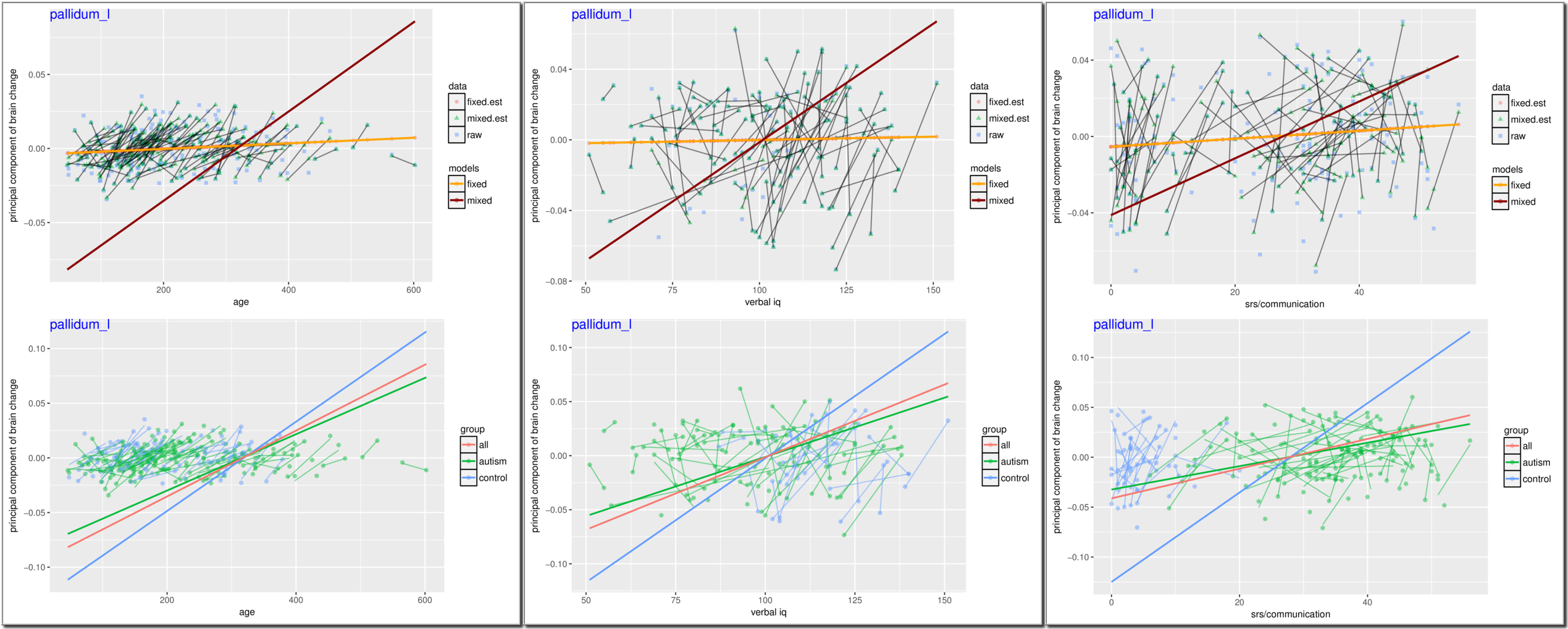
Relationships between longitudinally changing covariates ($$$x$$$-axis) and the primary longitudinal brain change ($$$y$$$-axis). Data from one of the regions of interest, pallidum (implicated to be enlarged in autism6), are presented. These relationships were estimated using our algorithms on the data with atleast three time points (since that gives us the needed minimum of two change values). For comparison, fixed effects models also were estimated and as expected (c.f., Fig. 1-right) the mixed effects models reveal interesting correlations. Notice that these non-zero slopes represent the rate of brain change per unit change in the clinical covariate. High resolution image available online.
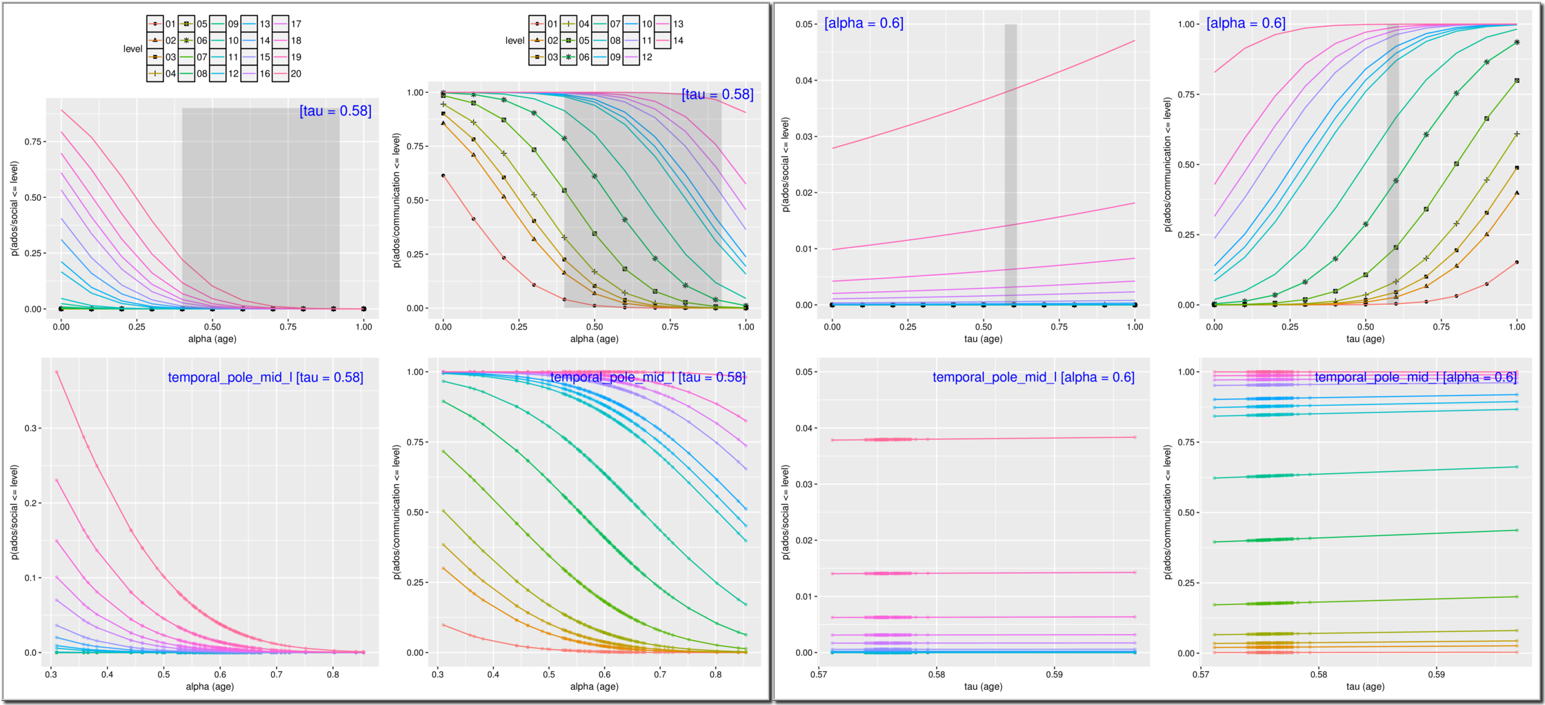
In addition, relationships between the subject-specific longitudinal effects (acceleration $$$\alpha$$$ and $$$time-shift$$$) and cross-sectionally available clinical covariates can also be examined. Data from the cumulative link models (CLMs) relating acceleration and time-shifts in temporal pole and a discrete subscale of autism-diagnostic-observation-schedule (ADOS) are presented. These 'onion plots' reveal cumulative likelihoods for different discrete levels of ADOS as a function of $$$\alpha$$$ and $$$\tau$$$. Effect of $$$\alpha$$$ (acceleration) (left) is in opposite direction to that of the onset of brain changes ($$$\tau$$$) (right). Top panel displays the model while the bottom panel displays data from temporal pole. High resolution image available online.
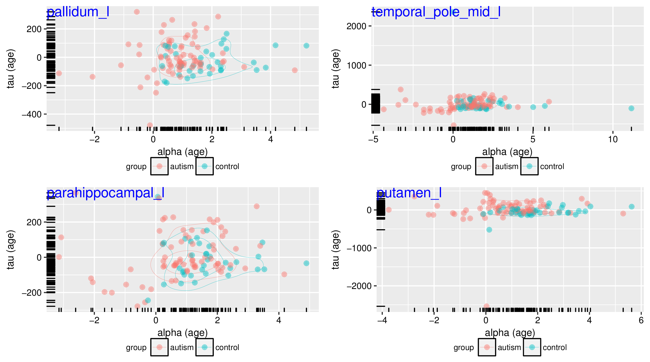
The mixed model parameters i.e. subject specific "trait" parameters ($$$\alpha$$$ and $$$tau$$$) can also offer a sensitive basis for classifying clinical diagnoses ("state" variables). Data from several different regions are shown where the samples are projected to the $$$\alpha$$$, $$$\tau$$$ space. It can be noticed in these plots that the longitudinal acceleration of brain change with age ($$$\alpha=\frac{\partial_t CDT}{\partial_t age}$$$) is mostly positive for controls while it is more spread and also negative in the autism group. This pattern was observed in many different regions of interest defined on the automated anatomical labeling (AAL) atlas. High resolution image available online.