3501
Bi-exponential modeling of prostate diffusion weighted MR imaging acquired using high b values: clinical evaluations of advanced post-processing methods1Department of Diagnostic Radiology, University of Turku, Turku, Finland, 2Department of Future Technologies, University of Turku, Turku, Finland, 3Turku PET Center, University of Turku, Turku, Finland, 4Department of Pathology, Turku University Hospital, Turku, Finland, 5Department of Urology, Turku University Hospital, Turku, Finland, 6Medical Imaging Center of Southwest Finland, Turku University Hospital, Turku, Finland
Synopsis
The aim of this study was to evaluate various mathematical methods for enhanced parameter estimation of bi-exponential DWI (12 b values 0-2000 s/mm2) of prostate cancer. Least Squares (LSQ), Bayesian Shrinkage (BS) and Maximum Penalized Likelihood Estimation (MPLE) fitting methods were evaluated in the terms of Coefficients of Variation (CV), Contrast to Noise Ratio (CNR) and the Area under the curve (AUC) between tumor and non-tumor prostate tissue. BS and MPLE methods improved AUC and CNR values of bi-exponential model parameters and also decreased CV values in comparison with the commonly used LSQ fitting method.
Introduction
Diffusion weighted MR imaging (DWI) is a non-invasive imaging technique that has extensively being used for the detection and characterization of prostate cancer (PCa) during the last decade.1,2 Voxel-wise signal fitting utilizing bi-exponential model has potential of extracting more information from the DWI signal that the commonly used monoexponential model.3 Bi-exponential model could provide parameter estimates with more clinically relevant information about the underlying tissue. Unfortunately this approach usually results in parametric maps that are corrupted by noise due to low signal-to-noise ratio (SNR) of the DWI. Recent developments in Bayesian bi-exponential model fitting 4,5 have claimed to overcome this obstacle by denoising the parametric maps of the bi-exponential model utilizing the neighboring voxel information.Materials and Methods
The study was approved by institutional review board and each patient with historically confirmed prostate cancer (PCa) included in the study provided written informed consent. The DWI was performed using a 3T MR scanner with a single shot spin-echo echo planar imaging, monopolar diffusion gradient scheme, and the following parameters: TR/TE 3141/51 $$$ms$$$, FOV 250 × 250 $$$mm^{2}$$$, slice thickness 5 $$$mm$$$, diffusion gradient timing (Δ) 24.5 $$$ms$$$, diffusion gradient duration (δ) 12.6 $$$ms$$$, diffusion time (Δ − δ/3) 20.3 $$$ms$$$, 12 b values of [number of signal averages]: 0 [2], 100 [2], 300 [2], 500 [2], 700 [2], 900 [2], 1100 [2], 1300 [2], 1500 [2], 1700 [3], 1900 [4], 2000 [4] $$$s/mm^{2}$$$. Prostate cancer lesions were delineated using whole mount prostatectomy sections as the “gold standard”. Voxel-wise fitting of bi-exponential model ($$$f, D_f, D_s$$$), eq.1,6 was performed by Least Squares fitting (LSQ), Bayesian Shrinkage (BS)4 and Maximum Penalized Likelihood estimation (MPLE)5 methods on whole prostate area including the lesions.
$${\bf{Y}}=c(fe^{-{\bf{b}}D_f}+(1-f)e^{-{\bf{b}}D_s})~~~~(1)$$
where $$$N$$$ is the number of b-values, signal vector $$${\bf{Y}}=(y_n)^{N}_{n=1}$$$ is the obtained signal model values estimated from the bi-exponential model Eq.(1), $$${\bf{b}}=(b_n)^{N}_{n=1}$$$ is the b value set, $$$c$$$ is the signal without diffusion weighting. $$$D_s$$$ is the slow diffusion component, $$$D_f$$$ is the fast decay component and $$$f$$$ is the fraction between fast and slow diffusion components. While LSQ method only estimates each voxel parameters individually, both BS and MPLE utilize spatial prior characteristics of surrounding voxels as a prior knowledge when fitting the model parameters for individual voxels. MPLE hyper parameter set (kernel size, constraints and the weighting penalty) were optimized while BS and LSQ did not required any prior parameter settings. The goodness of the methods’ fit were evaluated using parametric maps and Fitting errors. Furthermore Coefficients of Variation (CV), Contrast to Noise Ratio (CNR) and the Area under the curve (AUC) between each tumor and non-tumor prostate region was calculated and compared in-between the methods.
Results
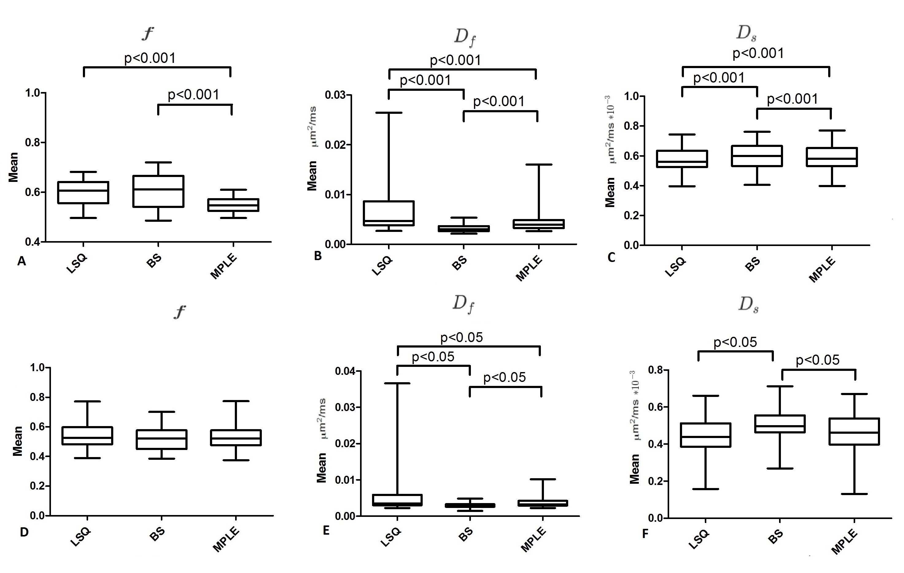
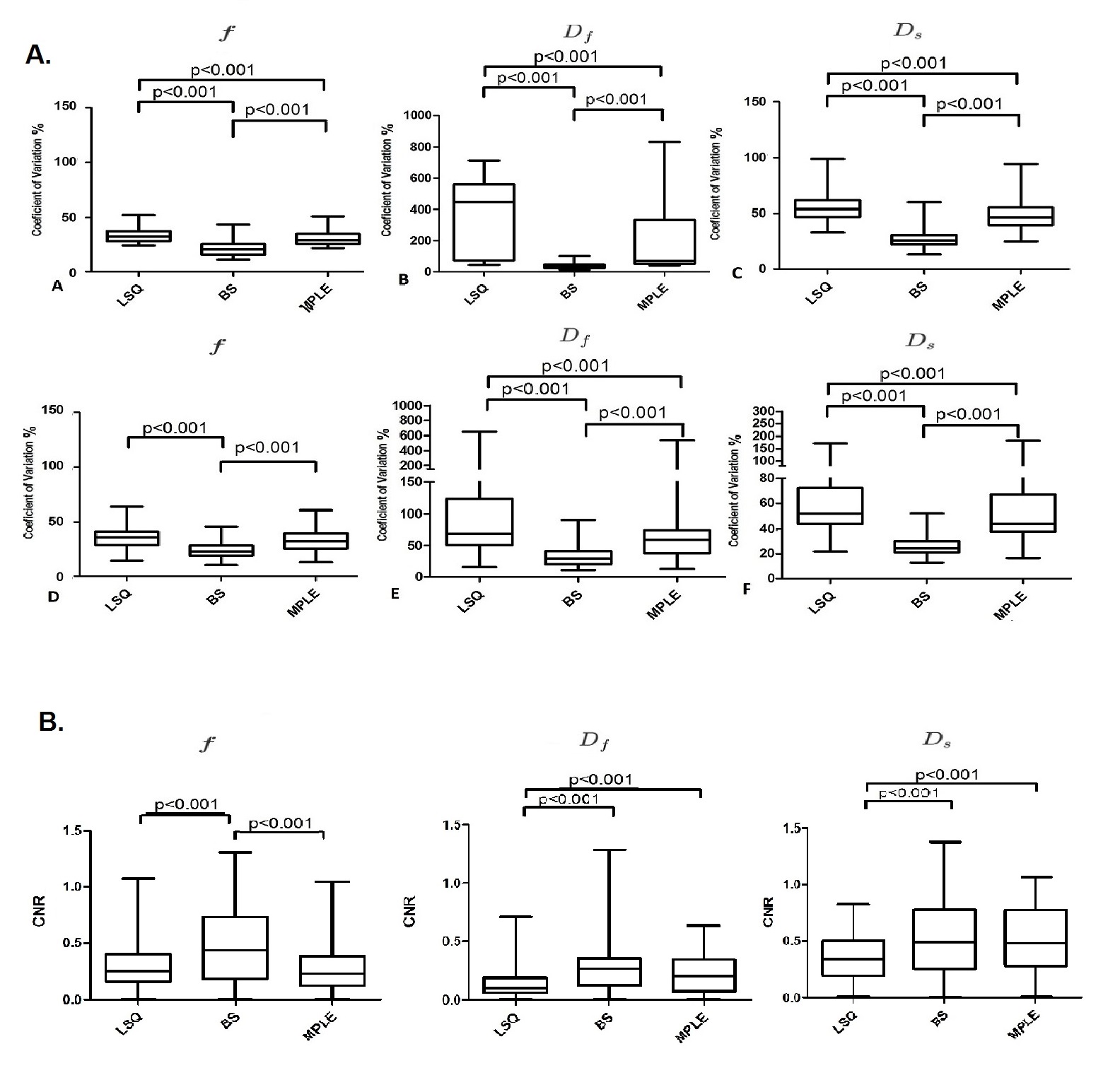
In total, 50 patients were included in final analyses. The tumor visibility was improved in both BS and MPLE for parametric maps (Figure1). The mean values of all estimated parameter values were lowest for BS and highest for LSQ (Figure2). The CV was significantly lower in all parameters’ estimation with BS method compared to other two methods ($$$p<0.05$$$) (see Figure 3.A). The BS and MPLE provided better CNR with the model parameter values $$$D_f$$$ and $$$D_s$$$ , compared with the LSQ and BS has significantly lower CNR for $$$f$$$ parameter (Figure 3.B).
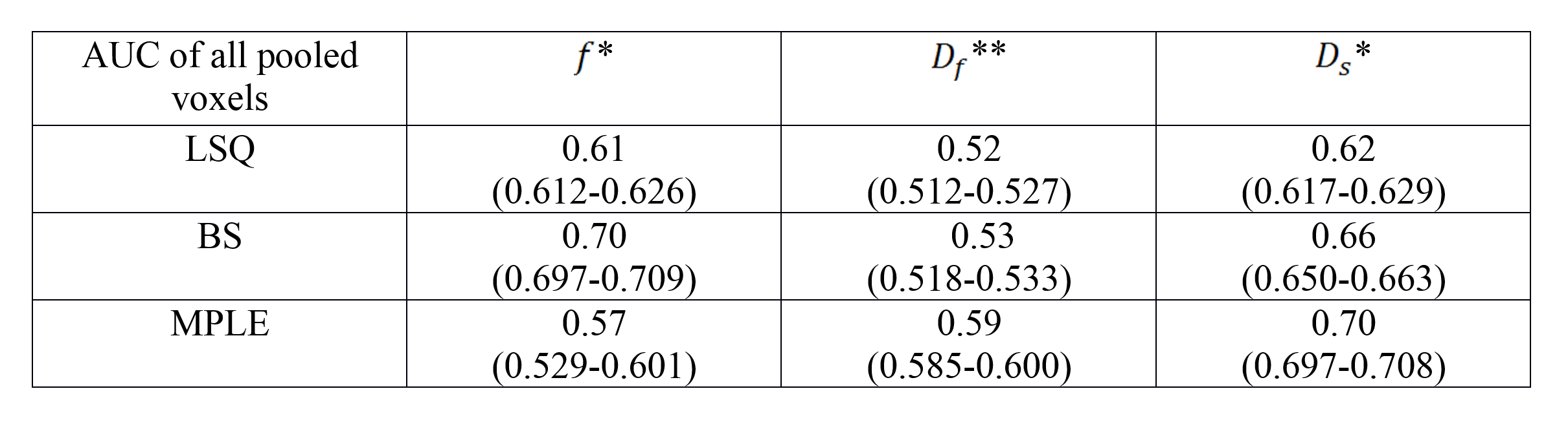
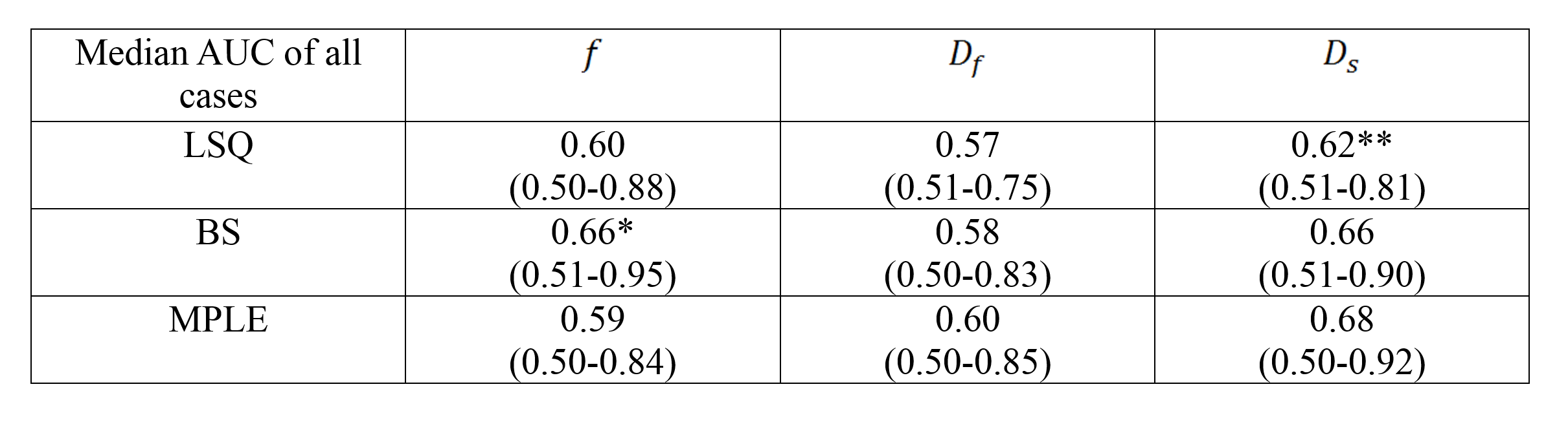
For classification performance between cancer and non-cancer tissue types when voxels of all 50 cases were pooled, the BS and MPLE method provided better AUC values than LSQ. The best classification performance was with MPLE method in $$$D_f$$$ and $$$D_s$$$ while classification performance for $$$f$$$ parameter was best with the Bayesian Shrinkage (Table 1). The AUC values calculated for each subject separately are shown in Table 2. Significant differences between methods were found in $$$f$$$ and $$$D_f$$$ parameters. Classification performance of $$$f$$$ was best with BS. For $$$D_f$$$ and $$$D_s$$$ the classification performance was better with BS and MPLE than with LSQ, where in $$$D_s$$$ the difference was statistically significant.
Discussion
To the best of our knowledge, bi-exponential parametric map enhancement using BS and MPLE methods, have not yet been evaluated for their use in prostate cancer studies. Our results showed that spatially constraint bi-exponential methods offer possibilities for improved quantification of prostate DWI. BS method should be used with caution because while it globally optimizes the model parameters, the information might get lost if the tumor to prostate ratio is very small.Conclusion
In conclusion, our results suggest that the presented advanced Bayesian based methods improves image contrast (CNR) and classification performance (AUC) in voxel-wise level of bi-exponential model which may lead to better detection and characterization of prostate cancer.Acknowledgements
No acknowledgement found.References
1. Padhani AR, Liu G, Mu-Koh D et al. Diffusion-weighted magnetic resonance imaging as a cancer biomarker: consensus and recommendations. Neoplasia 2009;11(2):102-125.
2. Shinmoto H, Oshio K, Tanimoto A et al. Biexponential apparent diffusion coefficients in prostate cancer. Magnetic Resonance Imaging 2009;27(3):355-359.
3. Le Bihan D, Breton E, Lallemand D, Aubin ML, Vignaud J, Laval-Jeantet M. Separation of diffusion and perfusion in intravoxel incoherent motion MR imaging. Radiology 1988;168(2):497-505.
4. Orton MR, Collins DJ, Koh D, Leach MO. Improved intravoxel incoherent motion analysis of diffusion weighted imaging by data driven Bayesian modeling. Magnetic resonance in medicine 2014;71(1):411-420.
5. Taimouri V, Afacan O, Perez-Rossello JM et al. Spatially constrained incoherent motion method improves diffusion-weighted MRI signal decay analysis in the liver and spleen. Medical physics 2015;42(4):1895-1903.
6. Clark CA, Le Bihan D. Water diffusion compartmentation and anisotropy at high b values in the human brain. Magn Reson Med 2000; 44:852-859.
Figures