Synopsis

Accurate delineation of anatomical boundaries on prostate MR is crucial for cancer staging and standardized assessment. Unfortunately, manual prostate segmentation is time consuming and prone to inter-rater variability while existing automated segmentation software is expensive and inaccurate. We demonstrate a novel fully-automated zonal prostate segmentation method that is fast and accurate using a convolutional neural network. The network is trained using a dataset of 149 T2-weighted prostate MR volumes that were manually annotated by radiologists. Our method improves upon prior related work, achieving a full-gland Dice score of 0.92 and zonal Dice score of 0.88.

Background

Methods

The dataset consists of 149 axial T2-weighted prostate MRI volumes from a publicly available dataset², of which 125 were reserved for training and 24 for testing. The authors manually classified each pixel in the dataset as non-prostate, transition zone, or peripheral zone, producing a set of ground-truth segmentation masks. Each volume was then scaled to a uniform height and width (256 x 256) and pixel intensities were normalized to values between zero and one on a per-volume basis. Data augmentation was performed by applying random transformations at batch time, including horizontal/vertical flip, rotation, and gaussian noise.

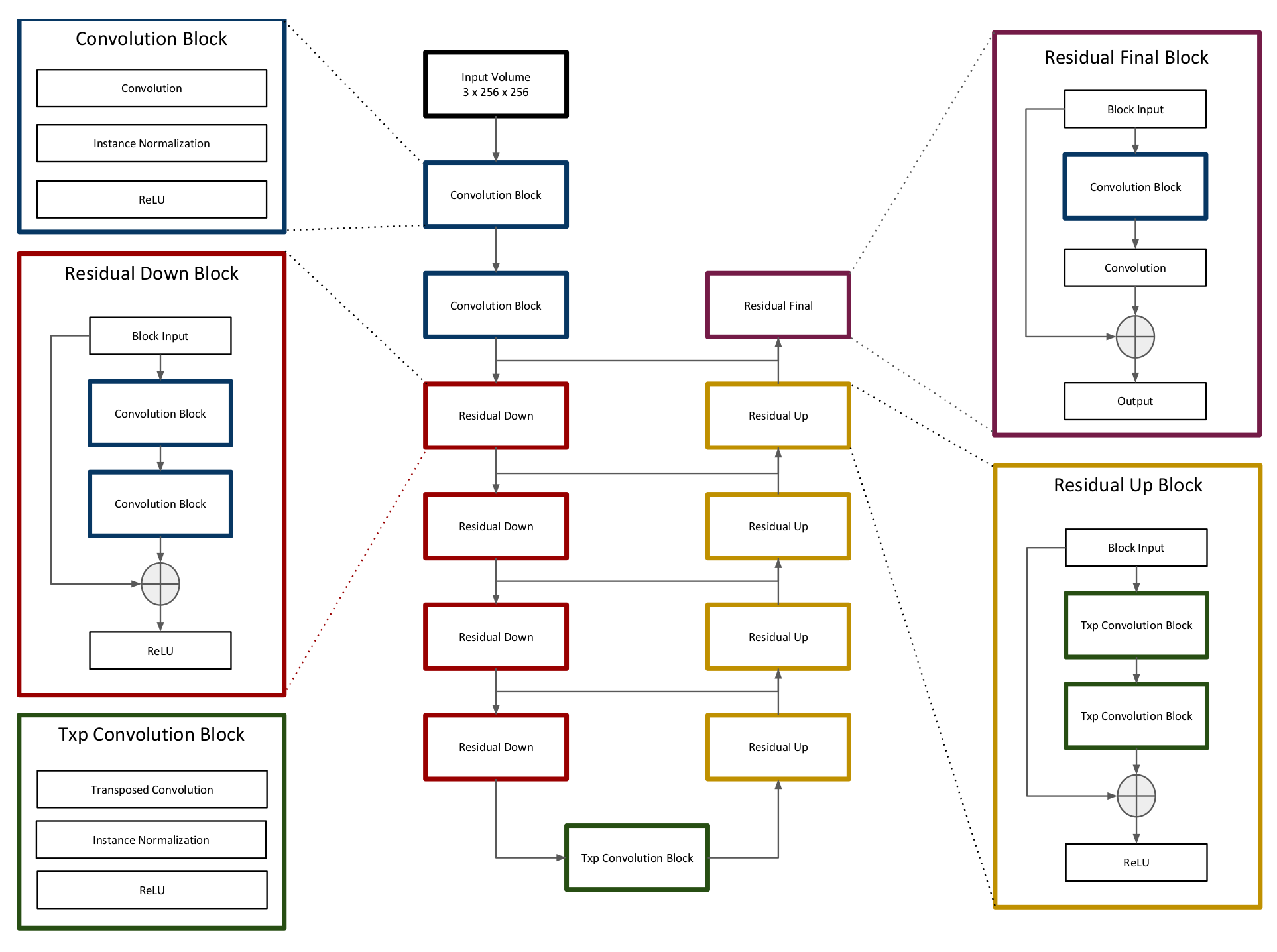
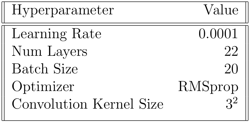
The model consists of a deep neural network based loosely on the popular U-net architecture³, which has become popular in recent years for excellent performance in various segmentation tasks. We modify the standard U-net architecture by adding residual modules, as demonstrated by Han⁴ (Figure 1). The model accepts subvolumes of size 3 x 256 x 256 (depth x height x width) and produces segmentation masks of size 3 x 3 x 256 x 256 (depth x num_classes x height x width). We refer to the model as “2.5D” because input subvolumes are three-dimensional while the network, including all convolution operators, is two-dimensional. The decision to use a 2.5D network as opposed to a 2D or 3D network was made to balance a desire to incorporate information from neighboring slices with hardware memory limitations. Model hyperparameters (Table 1) were chosen rationally and not by exhaustive search.

The dataset contains an inherent class imbalance in that most pixels are non-prostate. To overcome problems related to class balance, a weighted softmax function was used as part of the objective such that each pixel was scaled in proportion to its rarity. Model performance was evaluated by calculating the Dice coefficient (Equation 1) between generated segmentations and corresponding ground-truth segmentations in the test set. The total model score is the average of the Dice scores for each volume.$$(1) DCE = 2 |A ∩ B| / (|A| + |B|) $$

The network was built in python using the neural network library PyTorch. It was trained for 12 hours on a single graphics processing unit with 11 GB of video RAM.

Our institutional review board deemed this study exempt from institutional review due to the public and anonymized nature of the dataset.

Results and Discussion

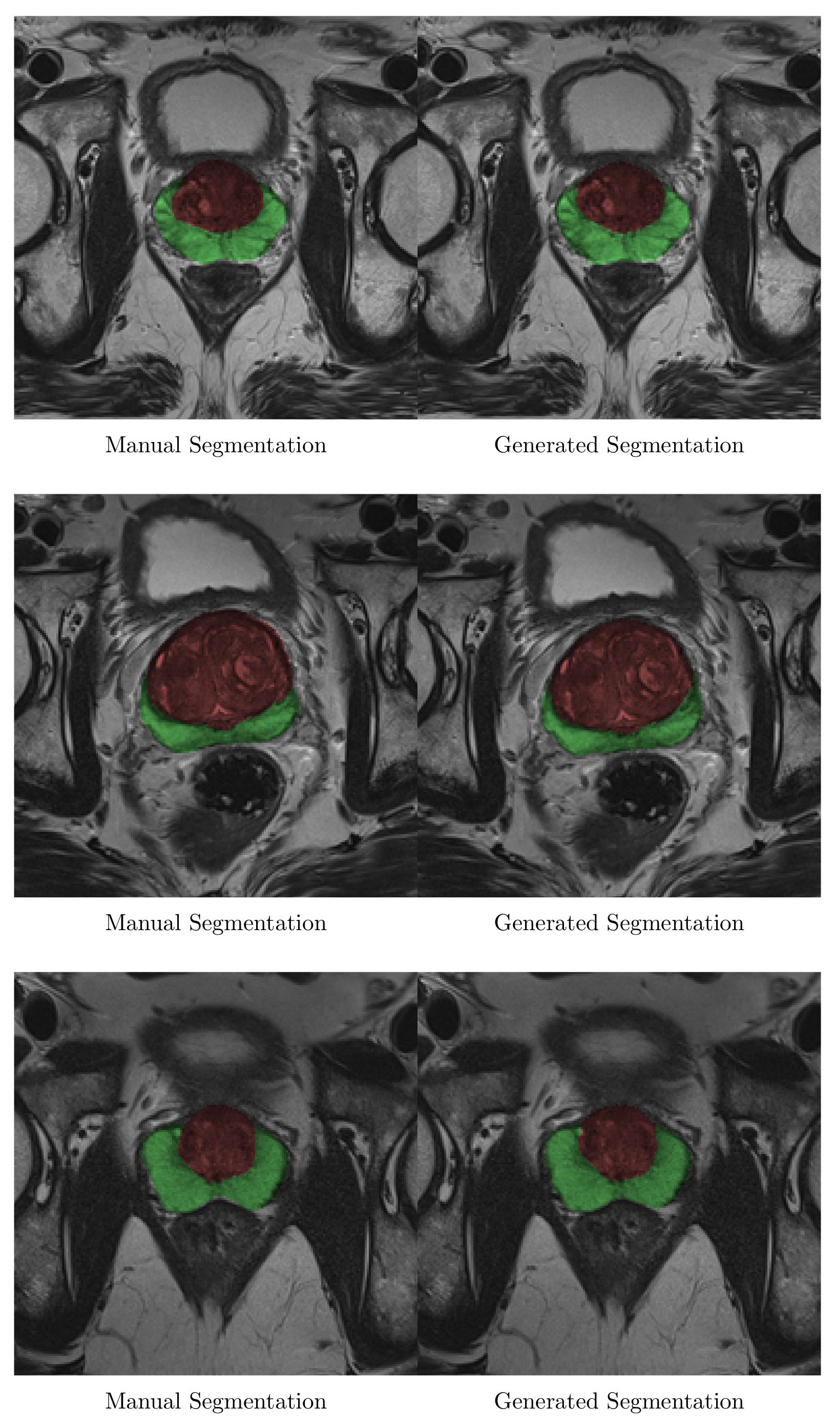
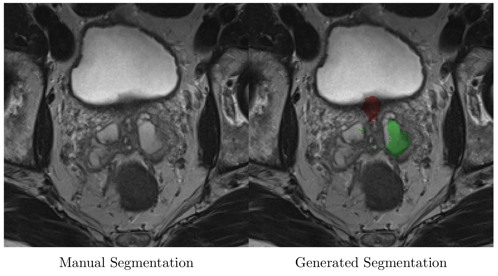
Sample output slices are shown in Figure 2. Mean whole-gland Dice coefficient was 0.92 (95% CI 0.91-0.93) for the test set and 0.97 (95% CI 0.97-0.97) for the training set. Mean zonal Dice coefficient was 0.88 (95% CI 0.87-0.89) for the test set and 0.95 (95% CI 0.95-0.95) for the training set. Processing time ranged from 0.5 to 1.2 seconds per volume. Model errors occurred when a pixel was misclassified. Errors were most common at the superior and inferior margins of the prostate, where volume averaging makes anatomical boundaries somewhat ambiguous (Figure 3).

These data suggest that our model is a viable alternative to manual segmentation and can be used as a replacement for existing automated methods. To our knowledge this represents an improvement over the best-performing prostate segmentation models in the literature^5,6. We credit the performance improvement to the use of a) a streamlined purely-residual architecture, b) instance normalization⁷ rather than batch normalization, which tends to perform poorly with small batch sizes, and c) weighted softmax to combat class imbalance. Limitations of this study include the relatively small size of the dataset in comparison to industrial-grade non-medical datasets, which undoubtedly contributed to the discrepancy between test and training set performance. Future work will focus on acquiring more data and integrating the model into clinical workflows. We also intend to experiment with newer model variants, including the recently introduced densely connected neural network architecture⁸.

Acknowledgements

References

1. Greenham, Stuart, et al. "Evaluation of atlas‐based auto‐segmentation software in prostate cancer patients." Journal of medical radiation sciences 61.3 (2014): 151-158.

2. Geert Litjens, Oscar Debats, Jelle Barentsz, Nico Karssemeijer, and Henkjan Huisman. "ProstateX Challenge data", The Cancer Imaging Archive (2017).

3. Ronneberger, Olaf, Philipp Fischer, and Thomas Brox. "U-net: Convolutional networks for biomedical image segmentation." International Conference on Medical Image Computing and Computer-Assisted Intervention. Springer, Cham, 2015.

4. Han, Xiao. "Automatic Liver Lesion Segmentation Using A Deep Convolutional Neural Network Method." arXiv preprint arXiv:1704.07239 (2017).

5. Clark, Tyler, et al. "Fully automated segmentation of prostate whole gland and transition zone in diffusion-weighted MRI using convolutional neural networks." Journal of Medical Imaging 4.4 (2017): 041307.

6. Jia, Haozhe, et al. "Prostate segmentation in MR images using ensemble deep convolutional neural networks." Biomedical Imaging (ISBI 2017), 2017 IEEE 14th International Symposium on. IEEE, 2017.

7. Ulyanov, Dmitry, Andrea Vedaldi, and Victor Lempitsky. "Instance normalization: The missing ingredient for fast stylization." arXiv preprint arXiv:1607.08022 (2016).

8. Huang, Gao, et al. "Densely connected convolutional networks." arXiv preprint arXiv:1608.06993 (2016).