3489
Cascaded 3D fully convolutional neural network for segmenting amygdala and its subnuclei1University of Wisconsin Madison, Madison, WI, United States
Synopsis
We address the problem of segmenting subcortical brain structures that have small spatial extent but are associated with many neuropsychiatric disorders and neurodegenerative diseases. Specifically, we focused on the segmentation of amygdala and its subnuclei. Most existing methods including deep learning based focus on segmenting larger structures and the existing architectures do not perform well on smaller structures. Hence we designed a new cascaded fully convolutional neural network with architecture that can perform well even on small structures with limited training data. Several key characteristics of our architecture: (1) 3D convolutions (2) deep network with small kernels (3) no pooling layers.
Introduction
The amygdala is a critical region of the “social brain”1, and is believed to be closely related to anxiety2 and autism3, but as a deep heterogenous cluster of subnuclei, surrounded by vasculature and sources of MRI field inhomogeneities, it remains an extremely difficult region to quantify by commonly-used automated methods. Additionally, animal models continue to differentiate subnuclei of the amygdala, identifying structural bases of fear generalization in basal and lateral nuclei distinct from output projections from centromedial regions. Therefore, a reliable quantitation of the amygdala and its substructures is urgently needed. Recently, deep learning methods such as convolutional neural networks (CNN) have demonstrated state-of-the-art performance in object-level and pixel-level classification4, due to its ability to learn hierarchical features from training data5. Although CNNs have already been investigated in several medical applications, most of the current approaches failed to incorporate the full spatial extent during segmentation and use only a slice-by-slice 2D neighborhoods6,7 for lowering the computation and memory costs. Our work, building on previous work8, takes advantage of the full 3D spatial neighborhood information by using 3D patches as inputs for the network. Our architecture for segmenting the amygdala has exhibited significant increase in accuracy compared to Freesurfer and FSL's FIRST, and better results than other recent deep learning techniques9,10, without requiring any post-processing steps. To the best of our knowledge, this work is also the first fully convolutional neural network (FCN) model for segmenting the subnuclei of the amygdala. Our architecture for segmenting these 10 subfields has also demonstrated very promising results.Methods
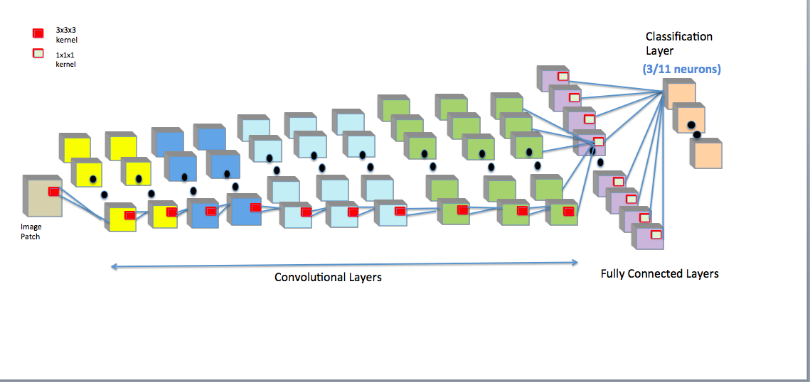
The design and training of our networks were based on the LiviaNET framework7. The pre-processing step involves the standard skull-stripping for extracting the brain and volume-wise intensity normalization from the $$$T_1$$$-weighted MRI. We extracted patches of size $$$25\times 25\times 25$$$ from both the training set and the corresponding ground truth labels. Patches were randomly and uniformly sampled from the entire brain without any special emphasis on the regions of interests (ROIs). The key technical contribution is the design of cascaded FCN which uses the same architecture but learns different weights based on different tasks. The FCN was independently trained for (1) segmenting the full amygdala and (2) segmenting its subnuclei. Note that this is different from a hierarchical organization of tasks. The architecture (Fig. 1) consists of 10 successive convolutional layers with kernel size $$$3\times 3\times 3$$$ and a classification layer (a set of $$$1\times 1\times 1$$$ convolutional kernels) with softmax activation function for obtaining normalized probabilities for each class that each voxel belongs to. The number of kernels on each layer is $$$20,20,30,30,50,50,50,75,75,75,100,$$$ respectively. We employed negative likelihood as cost function, which is optimized using the RMSprop11 optimization method with the decay rate 0.9. The initial learning rate was set to 0.001, decaying 0.5 after every epoch. Each epoch consists of 2 sub-epochs. To avoid bias, we employed the leave-one-out cross validation scheme for our experiments, i.e., for each epoch, 11 subjects were used for training and the left one was for validation. This was repeated 12 times until every subject's segmentation had been used for validation.The network for each task was separately trained for 20 epochs. The similarity and discrepancy of the automatic and manual segmentation were evaluated using the Dice Similarity Coefficient (DSC)12 which is defined as the following for automatic segmentation $$$A$$$ and manual segmentation $$$M$$$, $$$DSC(A, M) = \frac{2|A\cap M}{|A|+|M|}$$$.$$$\mathtt{DSC}$$$ values are in the $$$[0,1]$$$ range, where 1 indicates 100% overlap with the ground truth, and 0 indicates no overlap.Results
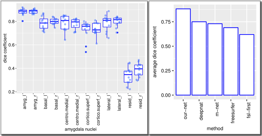
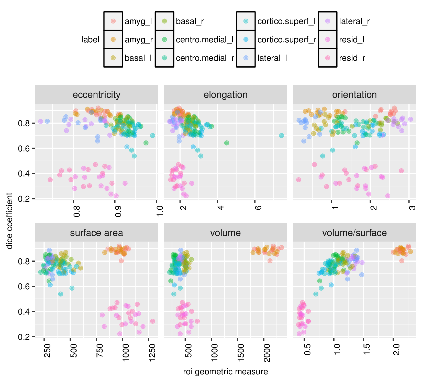
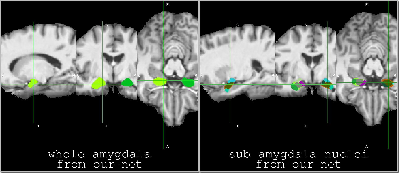
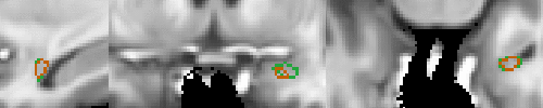
Our architecture is presented in Fig.1. Our method shows excellent performance in segmenting the two whole amygdalae with the mean dice scores: 0.88 and 0.89, respectively. It also shows very promising results in segmenting the subnuclei (Fig.2). Fig.3 shows the effects of geometric features of the subfields on the dice score. Figs.4,5 show some representative segmentation results.Conclusion and discussion
We found that the volume-to-surface ratio is inversely related to the difficulty of the segmentation, which could account for the lower accuracy yielded when segmenting the residue regions of the amygdala. For example, this difficulty persisted even with skip connections of intermediate layers. We will also validate our method on other amygdala dataset. These difficulties could potentially be tackled by (1) exploring the advantage of dilated convolution13 for enlarging the receptive field to incorporate knowledge from even bigger spatial extents, (2) applying data augmentations methods such as affine transformations and generative adversarial networks (GANs)14 to address the issue of limited data size and make the segmentation more robust, (3) enhance the training data for further generalization to data acquired from different $$$T1$$$-weighted sequences and different scanners.Acknowledgements
NIH grants U54-HD090256 and P50-MH100031 are acknowledged.References
1. Nacewicz BM, Angelos L, Dalton KM, Fischer R, Anderle MJ, Alexander AL, Davidson RJ (2012) Reliable non-invasive measurement of human neurochemistry using proton spectroscopy with an anatomically defined amygdala-specific voxel. Neuroimage 59(3):2548–2559
2. Shin, L.M. & Liberzon, I. The neurocircuitry of fear, stress, and anxiety disorders. Neuropsychopharmacology 35, 169-191 (2010)
3. Baron-Cohen, S., Ring, H.A., Bullmore, E.T., Wheelwright, S., Ashwin, C., & Williams, S.C.R. ( 2000). The amygdala theory of autism. Neuroscience and Biobehavioral Reviews, 24, 355–364.
4. Krizhevsky, I. Sutskever, and G. E. Hinton. Imagenet classification with deep convolutional neural networks. In Advances in Neural Information Processing Systems 25, pages 1106–1114, 2012.
5. Lecun, Y., Bengio, Y. & Hinton, G. Deep Learning. Nature 521, 436-444(2015)
6. Abhijit Guha Roy, Sailesh Conjeti, Debdoot Sheet, Amin Katouzian, Nassir Navab, Christian Wachinger:Error Corrective Boosting for Learning Fully Convolutional Networks with Limited Data.CoRR abs/1705.00938 (2017)
7. O. Ronneberger, P. Fischer, and T.Brox, U-net: Convolutional networks for biomedical image segmentation, in MICCAI, pp.234-241, Springer, 2015
8. Dolz J, Desrosiers C, Ben Ayed I. 3D fully convolutional networks for subcortical segmentation in MRI: A large-scale study. NeuroImage (2017).
9. Wachinger, C., Reuter, M., Klein, T.: DeepNAT: deep convolutional neural network for segmenting neuroanatomy. NeuroImage (2017)
10. Mehta, R., and Sivaswamy, J., 2017. M-net: A Convolutional Neural Network for deep brain structure segmentation. In Biomedical Imaging (ISBI 2017), 2017 IEEE 14th International Symposium on (pp. 437-440). IEEE
11. Tieleman, Tijmen and Hinton, Geoffrey. Lecture 6.5-rmsprop: Divide the gradient by a running average of its recent magnitude. COURSERA: Neural Networks for Machine Learning, 4, 2012.
12. L. R. Dice, Measures of the amount of ecologic association between species, Ecology 26 (3) (1945) 297-302
13. F. Yu and V. Koltun, Multi-scale context aggregation by dilated convolutionals, in ICLR, 2016.
14. Goodfellow, Ian J., Pouget-Abadie, Jean, Mirza, Mehdi, Xu, Bing, Warde-Farley, David, Ozair, Sherjil, Courville, Aaron C., and Bengio, Yoshua. Generative adversarial nets. NIPS, 2014.
Figures