3487
Fully Automatic Proximal Femur Segmentation in MR Images using 3D Convolutional Neural Networks1Center for Data Science, New York University, New York, NY, United States, 2Department of Radiology, Center for Musculoskeletal Care, New York University Langone Medical Center, New York, NY, United States, 3Osteoporosis Center, Hospital for Joint Diseases, New York University Langone Medical Center, New York, NY, United States, 4Courant Institute of Mathematical Science & Center for Data Science, New York University, New York, NY, United States, 5Department of Radiology, Center for Advanced Imaging Innovation and Research (CAI2R) and Bernard and Irene Schwartz Center for Biomedical Imaging, New York University Langone Medical Center, New York, NY, United States, 6The Sackler Institute of Graduate Biomedical Sciences, New York University School of Medicine, New York, NY, United States
Synopsis
MRI has been successfully used in structural imaging of trabecular bone micro architecture in vivo. In this project, we develop supervised convolutional neural network for automatically segmental proximal femur from structural MR images. We found that the proposed method provides accurate segmentation without any post-processing, bringing trabecular bone micro architecture analysis closer to clinical practice.
Introduction
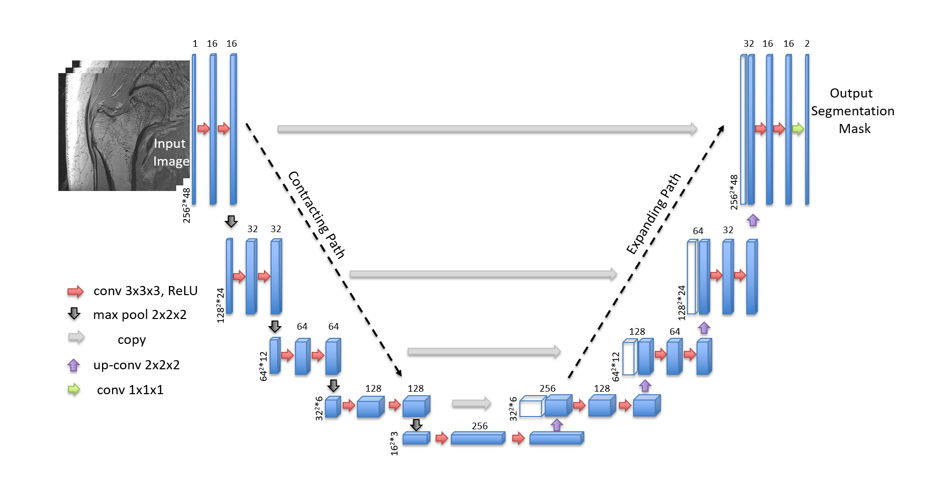
The segmentation of trabecular bone is required for measuring bone quality and assessing fracture risk precisely. Manual segmentation of the proximal femur is time-intensive, limiting the use of MRI measurements in clinical practice. To overcome this bottleneck, a robust automatic proximal femur segmentation method is necessary. In previous studies, hybrid image segmentation approaches including thresholding and 3D morphological operations 1 as well as statistical shape models 2 and deformable models 3,4 have been used for segmenting of the proximal femur from MR images. Several deep convolutional neural network (CNN) architectures have recently been successfully used in medical research for image segmentation 5-8. Recently, CNN architectures based on 2D convolutions for proximal femur segmentation have been proposed 9-10. In this work, we investigated the extension of 3D U-net architecture 11 with padded convolutions and max-pooling layers for automatic proximal femur segmentation.Methods
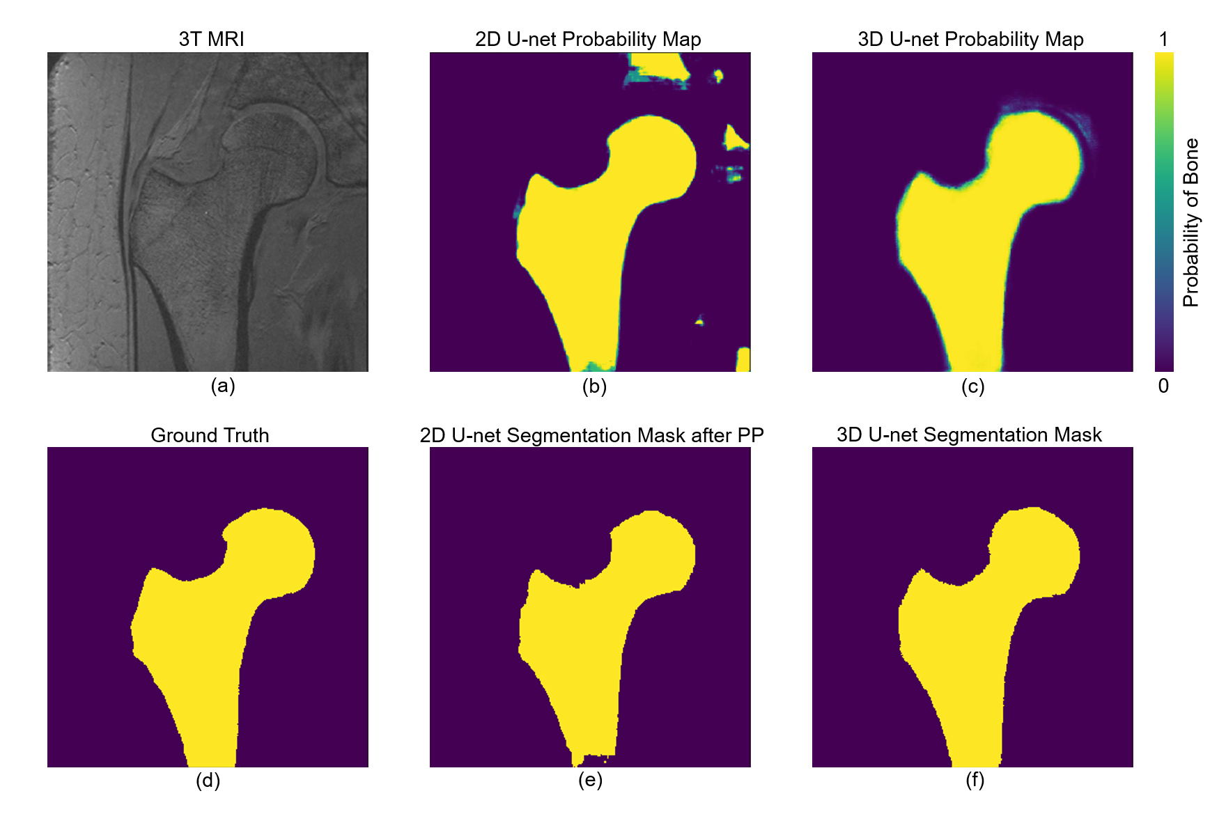
We used proximal femur microarchitecture MR images obtained from a clinical 3T MRI scanner (Skyra, Siemens, Erlangen) using commercial arrays (18-elements Siemens flexible array and 8-elements from the Siemens spine array). Images were obtained from 86 subjects using 3D FLASH sequence with following parameters: TR/TE=31/4.92ms; flip angle, 25; in-plane voxel size, 0.234×0.234 mm; section thickness, 1.5mm; number of coronal section, 60; acquisition time, 25 minutes 30 seconds; bandwidth, 200 Hz/pixel. Segmentation of the proximal femur is done by manual selection of the periosteal or endosteal borders of bone on MR images by an expert under the guidance of a musculoskeletal radiologist (Figure 5 (d)).
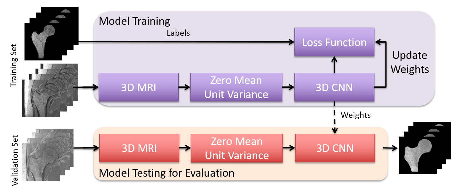
Figure 1 illustrates the workflow of our proposed segmentation algorithm. We used a supervised deep CNN for automatic fracture risk assessment based on the 3D U-net architecture (Figure 2). Compared with the 2D U-net, the 3D U-net facilitates the slice information more effectively via convolutions applied to z-axis as well. This enables the information from adjacent slides to be used during training which results in higher segmentation accuracy.
To evaluate the generalization ability of models, we performed 4-fold cross validation. We randomly partitioned our data into four subsets. Of these four subsets, one was used as a validation set and the other three were used as a training set. We do this four times and compute the aggregate statistics.
Convolutional kernel weights were initialized by Xavier and He initialization 12-13. For non-linearly transforming the data during modeling, rectifier linear units (ReLU) 14 were used. Since the background constitutes a large portion of the images, we used weighted cross entropy to balance contributes from different classes, where the weights are computed from the ground truth of training data. For the 2D U-net performance comparison, MR images were fed by combining 3 consecutive slices. In the case of 3D U-net, the central part of MR images (48 slices: covering the proximal femur) were used as an input to CNN. Experiments were conducted on a server using an NVIDIA 16GB Tesla P100 GPU card.
Results
In order to reduce training time for comparing various feature and layer sizes, we downsample data on both x- and y- axes using cubic spline interpolation and thus fewer convolution operations are needed in each layer. Experimental results show that reducing x- and y- axes from 512 to 256 results in 1/6 training time per epoch (from 30 minutes to 5 minutes). We used data with resolution 256x256x48 images for our analysis.
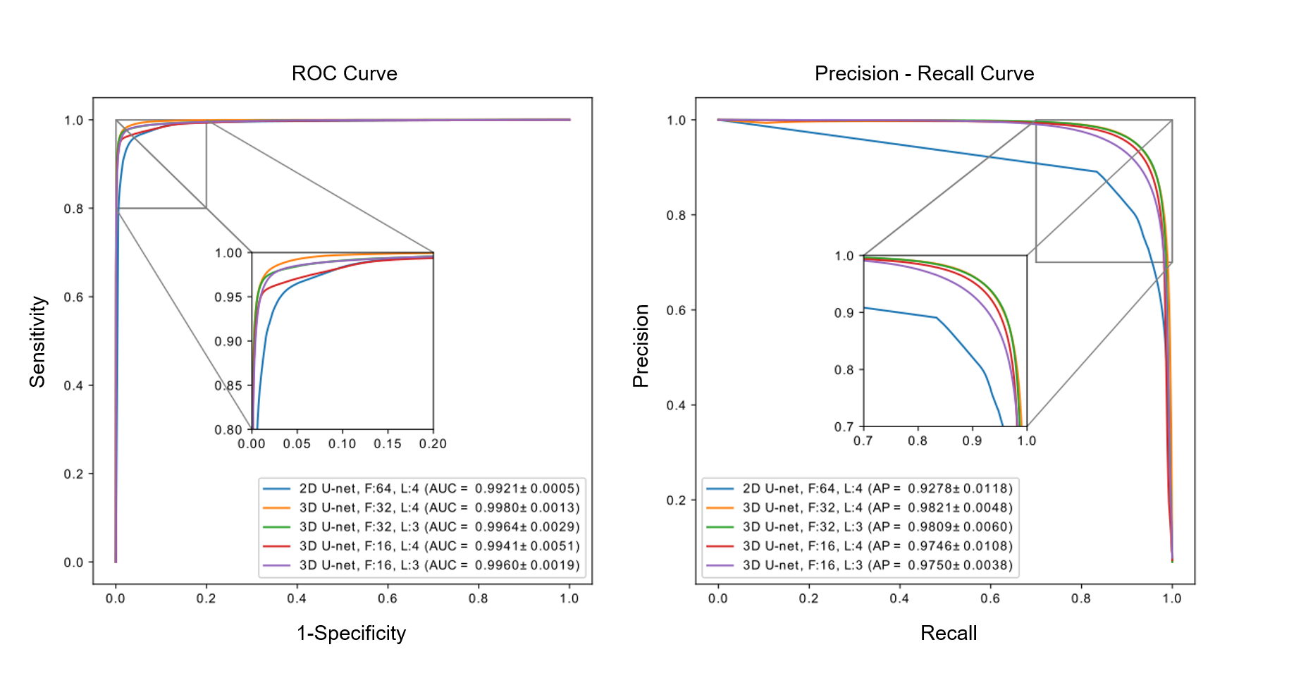
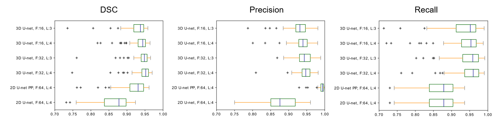
ROC and precision-recall curve analysis (Figure 3) of 2D and 3D models on the validation set show a high accuracy of the best 3D U-net, using 4 layers and 32 features, with area under the ROC curve (AUC) =0.9980±0.0013 and average precision from precision-recall curve (AP) =0.9821±0.0048. This significantly exceeds those of the 2D U-net which achieved AUC =0.9921±0.0005 and AP =0.9278±0.0118. The 3D U-net also reached the highest dice similarity coefficient (DSC) score (0.9395±0.0536) among these models. Individual scores obtained from validation subjects are illustrated in Figure 4. Segmentation results for different network architectures on a sample subject are presented in Figure 5.
Discussion and Conclusions
We implemented the 3D U-net CNN architecture for automatic segmentation of the proximal femur from MR images. Experimental results show that the 3D U-net surpasses the 2D U-net with or without post-processing steps, bringing the use of proximal femur MRI measurements closer to clinical practice.Acknowledgements
This work was supported in part by NIH R01 AR066008 and NIH R01 AR070131 and was performed under the rubric of the Center for Advanced Imaging Innovation and Research (CAI2R, www.cai2r.net), an NIBIB Biomedical Technology Resource Center (NIH P41 EB017183). We gratefully acknowledge the support of NVIDIA Corporation with the donation of a GPU for this research.References
1. R. a. Zoroofi, T. Nishii, Y. Sato, N. Sugano, H. Yoshikawa, and S. Tamura, “Segmentation of avascular necrosis of the femoral head using 3-D MR images.,” Computerized medical imaging and graphics : the official journal of the Computerized Medical Imaging Society, vol. 25, no. 6, pp. 511–21, 2001.
2. J. Schmid, J. Kim, and N. Magnenat-Thalmann, “Robust statistical shape models for MRI bone segmentation in presence of small field of view,” Medical Image Analysis, vol. 15, no. 1, pp. 155–168, 2011.
3. J. Schmid and N. Magnenat-Thalmann, “MRI Bone Segmentation Using Deformable Models and Shape Priors,” in Medical Image Computing and Computer-Assisted Intervention MICCAI 2008: 11th International Conference, New York, NY, USA, September 6-10, 2008, Proceedings, Part I (D. Metaxas, L. Axel, G. Fichtinger, and G. Székely, eds.), pp. 119–126, Berlin, Heidelberg: Springer Berlin Heidelberg, 2008.
4. S. Arezoomand, W. S. Lee, K. S. Rakhra, and P. E. Beaulé, “A 3D active model framework for segmentation of proximal femur in MR images,” International Journal of Computer Assisted Radiology and Surgery, vol. 10, no. 1, pp. 55–66, 2015.2
5. A. Prasoon, K. Petersen, C. Igel, F. Lauze, E. Dam, and M. Nielsen, “Deep feature learning for knee cartilage segmentation using a triplanar convolutional neural network,” in International conference on medical image computing and computer-assisted intervention, pp. 246–253,Springer, 2013.
6. S. Pereira, A. Pinto, V. Alves, and C. A. Silva, “Brain tumor segmentation using convolutional neural networks in mri images,” IEEE transactions on medical imaging, vol. 35, no. 5, pp. 1240–1251, 2016.
7. M. Lai, “Deep learning for medical image segmentation,” arXiv preprint arXiv:1505.02000, 2015.
8. R. Cheng, H. R. Roth, L. Lu, S. Wang, B. Turkbey, W. Gandler, E. S. McCreedy, H. K. Agarwal, P. L. Choyke, R. M. Summers,et al., “Active appearance model and deep learning for more accurate prostate segmentation on mri.,” in Medical Imaging: Image Processing, p. 97842I, 2016.
9. C. M. Deniz, S. Hallyburton, A. Welbeck, S. Honig, K. Cho, and G. Chang, “Segmentation of the proximal femur from MR images using deep convolutional neural networks,” CoRR, vol. abs/1704.06176, 2017.
10. S. Hallyburton, G. Chang, S. Honig, K. Cho, and C. M. Deniz, “Automatic segmentation of mr images of the proximal femur using deep learning,” Proceedings 25th Scientific Meeting, ISMRM, Hawaii, p. 3986, 2017.
11. Ö. Çiçek, A. Abdulkadir, S. S. Lienkamp, T. Brox, and O. Ronneberger, “3d u-net: learning dense volumetric segmentation from sparse annotation,” in International Conference on Medical Image Computing and Computer-Assisted Intervention, pp. 424–432, Springer, 2016.
12. X. Glorot and Y. Bengio, “Understanding the difficulty of training deep feedforward neural networks,” in Proceedings of the Thirteenth International Conference on Artificial Intelligence and Statistics, pp. 249–256, 2010.
13. K. He, X. Zhang, S. Ren, and J. Sun, “Delving deep into rectifiers: Surpassing human-level performance on imagenet classification,” CoRR, vol. abs/1502.01852, 2015.
14. V. Nair and G. E. Hinton, “Rectified linear units improve restricted boltzmann machines,” in Proceedings of the 27th international conference on machine learning (ICML-10), pp. 807–814, 2010.
Figures