3460
Feature Extraction using Convolutional Networks for Identifying Carotid Artery Atherosclerosis Patients in a Heterogeneous Brain MR Dataset1Departments of Radiology and Clinical Neuroscience, Hotchkiss Brain Institute, University of Calgary, Calgary, AB, Canada, 2Biomedical Engineering, University of Calgary, Calgary, AB, Canada, 3Calgary Image Processing and Analysis Centre, Foothills Medical Centre, Calgary, AB, Canada
Synopsis
Analysis of pathology in patients from heterogeneous datasets using machine learning techniques provide valuable information for identifying patients with carotid artery atherosclerosis disease. We propose and evaluate a method to automatically identify these patients based only on MR brain imaging findings in a dataset also containing multiple sclerosis patients and healthy control subjects. The features extracted using convolutional networks were discriminative, showing high accuracy rates (>96%) to distinguish between the three classes: atherosclerosis patients, multiple sclerosis patients or healthy controls. The method may help specialists in the diagnosis (specially in critical cases), and evaluation of disease activity.
Introduction
Manual extraction of information from large MR datasets is time-consuming and prone to errors due to intra- and inter-operator variability. These challenges in brain MR image analyses have stimulated the development of computer-assisted diagnosis technique, which through algorithms including machine learning (ML)-based approaches, aim to aid disease diagnosis and make it faster.1,2,3 We propose a ML technique to identify patients with carotid artery atherosclerosis (CA) from a cohort of MR brain images also containing patients diagnosed with multiple sclerosis (MS; serving here as positive controls), and healthy subjects (negative controls). We hypothesize the difference in white matter hyperintensities (WMH) will enable this discrimination. This method may be used to provide more complete information about the patient as a computer-aided diagnosis tool (CAD).Methods
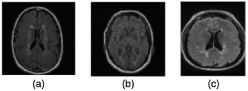
Experiments were performed on a dataset containing T2-weighted FLAIR sequence acquired on a 3T scanner (Discovery 750; GE Healthcare, Waukesha, WI) from 19 atherosclerosis patients (recruited by the Canadian Atherosclerosis Imaging Network4 with 3 mm slice thickness, TR = 9,700ms, TE =140 ms and TI = 2,200ms), 19 MS patients, and 19 healthy controls through the Calgary Normative Study5 using similar acquisition parameters. All subjects including the healthy subjects presented varying amounts of WMHs (Figure 1).
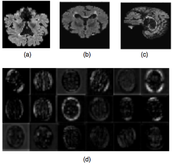
Initial steps standardize the MR images to make sure that the classification rates achieved by the proposed method are related to the presence/absence of pathology and not simply due to MR variability. We applied an N4 non-uniformity correction,6 brain extraction using the FSL package,7 brain cropping, intensity normalization to [0,255], and image resizing to (48,48,48). The convolutional features were computed by using a VGG16 network with pre-trained imagenet weights.8 For each MR volume, the convolutional features were computed in the central 2D axial, sagittal and coronal slices (Figure 2). For each of these three views, 25,088 convolutional features were computed and combined generating a feature vector of 75,264 features.
These features were used to
classify the participant groups using two different approaches: 1) distinguishing
normal from MS from CA in one step (3-label classification); or 2) using a
cascade classification, first distinguishing normal from abnormal samples using
binary classification, followed by the classification of the different types of
pathology, i.e., MS versus CA
patients (Figure 3). For both approaches, support-vector machine (SVM) models9
were used applying a 5-fold cross validation to split training and testing
datasets.10 The SVM parameters were chosen by using a grid-search
approach.11
Results
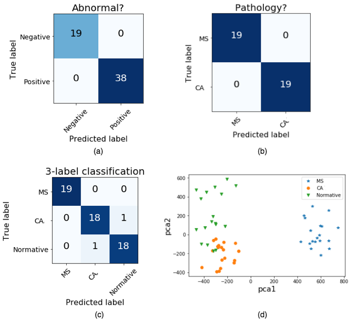
The two different approaches (single-staged, three-label classification: CA x MS x healthy images; and two-staged, binary classification: healthy x abnormal, followed by CA x MS) were evaluated quantitatively through confusion matrices. The three-label classification presented an accuracy of 96.5% to distinguish CA from positive controls (MS) and negative controls (normal subjects) (Figure 4c), while the two binary classifications presented no misclassifications (Figure 4a/b).
A qualitative evaluation was also provided through a 2D feature space visualization. Principal component analysis12 was applied to the convolutional features, and the top-two components were used to provide this 2D visualization (Figure 4d). This feature space shows that the 3 classes (CA, MS and normal controls) can be easily distinguished.
Discussion
The usage of robust convolutional features allows the discrimination between CA, MS and normal controls based on MR brain imaging information, even though the corresponding images present similar characteristics, such as the presence of WMHs, which are difficult to visually discriminate.
The proposed method using convolutional features to identify atherosclerosis patients from a heterogeneous dataset achieved high accuracy rates (>96%) when distinguishing CA from MS patients and healthy controls. The confusion matrices and feature space indicate that the convolutional features result in an easy-to-distinguish feature space. When using these robust, discriminative features, it is possible to choose a low-cost classifier because the discrimination is a straightforward task.
As expected, better results were achieved when using the two-staged cascade approach, since it represents a less complex task. This is also because we were using SVM classifiers, originally designed for binary classification tasks.13
Conclusion
The proposed method allows the proper identification of atherosclerosis patients in a dataset containing patients with other pathology (positive controls - MS), and normal subjects (negative controls). It may be used for CAD, suggesting possible disease diagnosis based only on MR imaging findings. Future experiments will include other pathologies and more heterogeneous datasets (i.e., including variable imaging protocols, scanner vendors, and field strength) to evaluate the robustness and reliability of this methodology.Acknowledgements
The authors would like to thank Hotchkiss Brain Institute for providing financial support.References
1. Despotovic I, Goossens B and Philips W. MRI segmentation of the human brain: Challenges, methods, and applications. Computational and Mathematical Methods in Medicine. 2015; 1(1): 1–23.
2. Leite M, Rittner L, Appenzeller S, et al. Etiology-based classification of brain white matter hyperintensity on magnetic resonance imaging. Journal of Medical Imaging. 2015; 2(1):014002.
3. Kwan R, Evans A and Pike G B. MRI simulation-based evaluation of image processing and classification methods. IEEE Transactions on Medical Imaging. 1999; 18(11):1085– 1097.
4. Tardif J, Spence J, Heinonen T, et al. Atherosclerosis imaging and the canadian atherosclerosis imaging network. The Canadian Journal of Cardiology. 2013;29 (3):297–303.
5. Tsang A, Lebel C, Bray S, et al. White Matter Structural Connectivity Is Not Correlated to Cortical Resting-State Functional Connectivity over the Healthy Adult Lifespan. Frontiers in Aging Neuroscience. 2017; 9:144.
6. Tustison N J, Avants B B, Cook P A, et al. N4ITK: improved N3 bias correction. IEEE Transactions on Medical Imaging. 2010;29(6): 1310 – 1320.
7. Jenkinson M, Beckmann C F, Behrens T E, et al. FSL. NeuroImage. 2012;62:782-90.
8. Shin H, Roth H, Gao M, et al. Deep convolutional neural networks for computer-aided detection: CNN architectures, dataset characteristics and transfer learning. IEEE Transactions on Medical Imaging. 2016;35(5):1285-1298.
9. Yichuan T. Deep learning using linear support vector machines. Proceedings of International Conference on Machine Learning, 2013.
10. Kohavi R. A study of cross-validation and bootstrap for accuracy estimation and model selection. Proceedings of International joint Conference on artificial intelligence. 1995; 14:1137–1145.
11. Bergstra J and Bengio Y. Random Search for Hyper-Parameter Optimization. Journal Machine Learning Research. 2012;13:281–305.
12. Jolliffe I. Principal Component Analysis. Springer Series in Statistics. 2002;2ed:28.
13. Hsu C H and Lin C J. A comparison of methods for multi-class support vector machines. IEEE Transactions on Neural Networks. 2002; 13:415-425.
Figures