Introduction

Breath-hold phase-contrast (bh-PC) MRI is a proven tool for assessment of blood flow and velocity through the great vessels¹. However, as a segmented acquisition, it may produce poor results in patients with irregular heart rhythm and/or dyspnea. One approach to address these problems is to perform real-time PC (rt-PC) MRI, as previously described using radial k-space sampling and compressed sensing (CS)². This pulse sequence, however, may produce considerable image artifacts (e.g., flicker through time) arising from a high data acceleration rate needed for achieving high temporal resolution (~40 ms). Temporal filters can be used to minimize aliasing artifacts, but such filters may cause temporal blurring and reduce velocity values^3,4. In this study, we sought to develop a CS reconstruction method that uses spatially varying regularization to reduce flickering artifacts without significant loss in accuracy, and evaluate its performance against clinical bh-PC MRI in patients undergoing aortic valve evaluation with cardiovascular MRI.

Methods

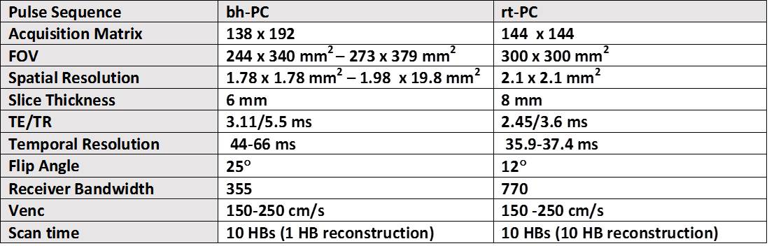
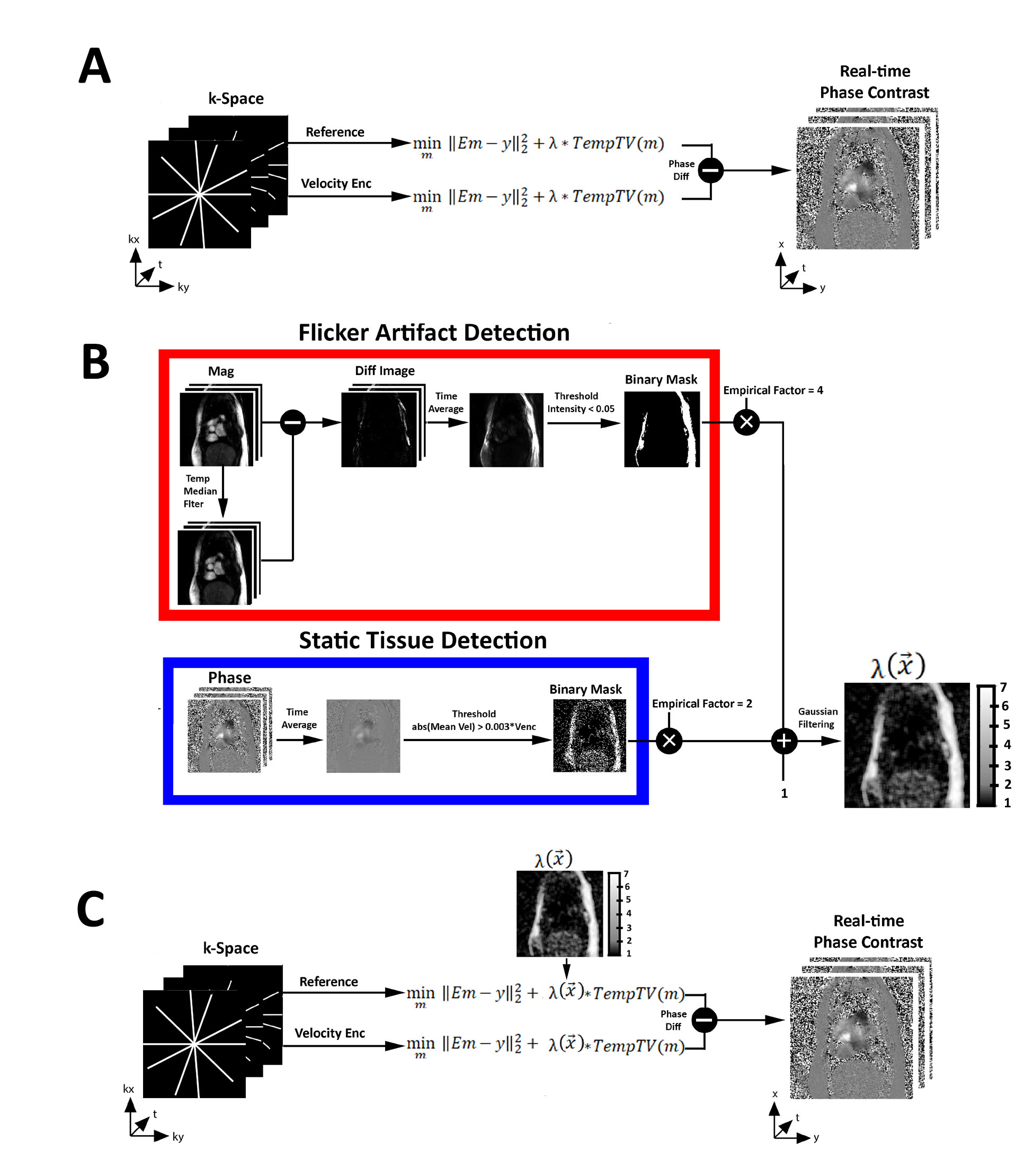
(Patient Enrollment) We scanned 6 patients (4 females, 2 males, mean age = 56.2 ± 17.1 years) with rt-PC and clinical bh-PC MRI on a 1.5T scanner (Siemens, Avanto) to image a plane that is superior to the aortic valve (i.e., ascending aorta). (Pulse Sequence) We developed a rt-PC MRI pulse sequence using radial k-space sampling³ with golden angle ratio = 111.23°⁵ and compared its performance against clinical bh-PC MRI (see Table 1 for relevant imaging parameters). (Image Reconstruction) The CS reconstruction was performed off-line on a workstation equipped with MATLAB (R2014a, The MathWorks). For CS reconstruction, after nonuniform fast Fourier transform⁶ and self-calibration⁷ of coil sensitivity maps, temporal total variation was used as the sparsifying transform⁸ with normalized regularization weight (λ)= 0.045 (or 4.5% of maximal signal). Note, the reference and velocity-encoded data were reconstructed separately. As shown in Figure 1, we explored two different regularization approaches: static and spatially varying. We adopted a previous described method⁹ to automatically derive a spatial mask that assigns high λ to locations generating high levels of flickering artifacts arising from the outer periphery (e.g., chest wall) and moderate levels of flickering artifact arising from static body tissues such as the liver (Figure 1). Briefly, locations causing flickering artifacts were detected by first applying a 1D median temporal filter to standard CS reconstructed magnitude images. The difference between the median filtered and original images was averaged over time to derive a normalized threshold value of 0.05 (Figure 1B). To remove flickering artifact arising from static body tissues, such locations were detected by averaging the phase images over time to derive a threshold value of 0.3% of velocity encoding (venc)(Figure 1B). We then combined the magnitude and phase masks with empirically derived factors 4 and 2, respectively, to derive a spatial varying λ map. Note, these empirical factors were derived from training data sets. (Qualitative Assessment) Two cardiologists and one radiologist graded the artifact level for CS reconstruction with static and spatially varying λ on a 5-point Likert scale (1: worst; 3: clinically acceptable; 5: best). (Velocity/Flow Quantification) For each data set, for both bh-PC and rt-PC MRI, a single region of interest (ROI) was drawn manually around the ascending aorta at a frame exhibiting high velocities (i.e., contrast). The ROI was then deformed through time using the Advanced Normalization Tools (ANTS)¹⁰. The rt-PC flow curves from multiple heat beats were average and compared to bh-PC flow curves using two tailed paired t-test and linear regression and Bland Altman analyses.

Results

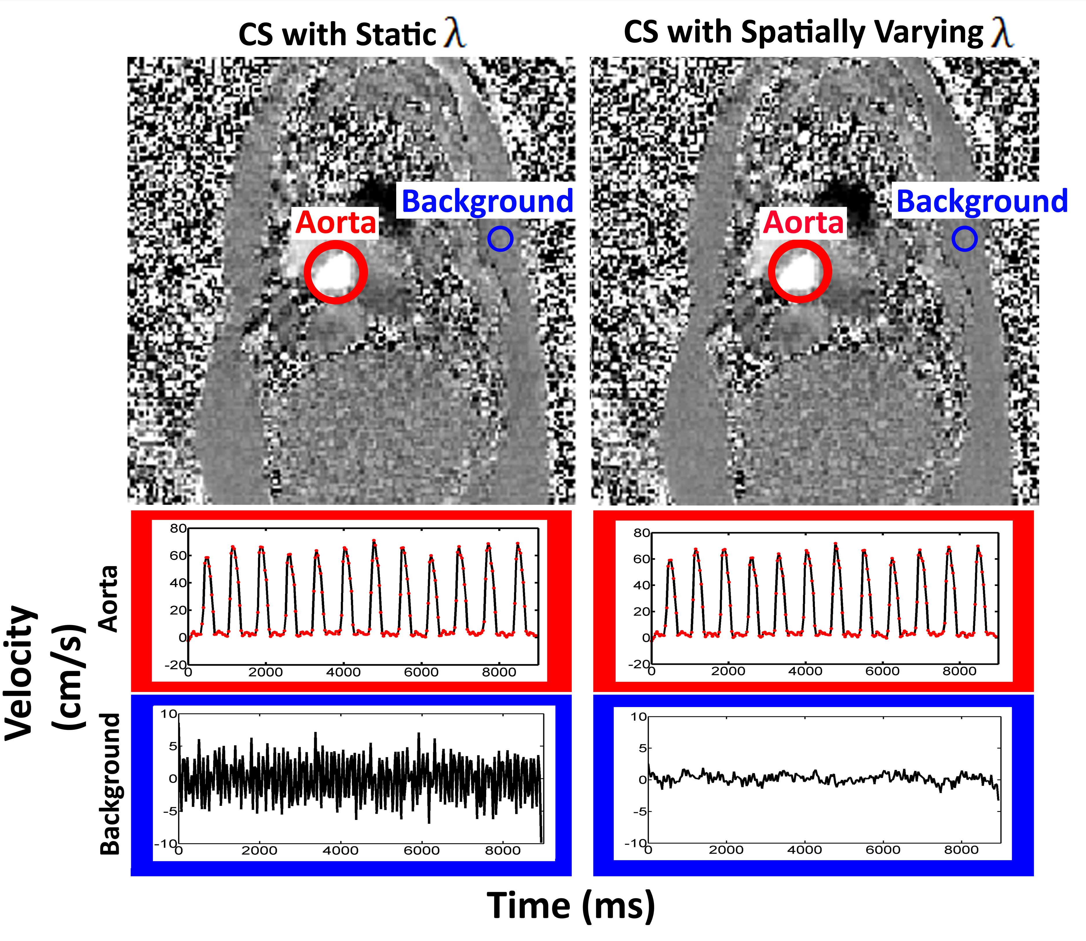
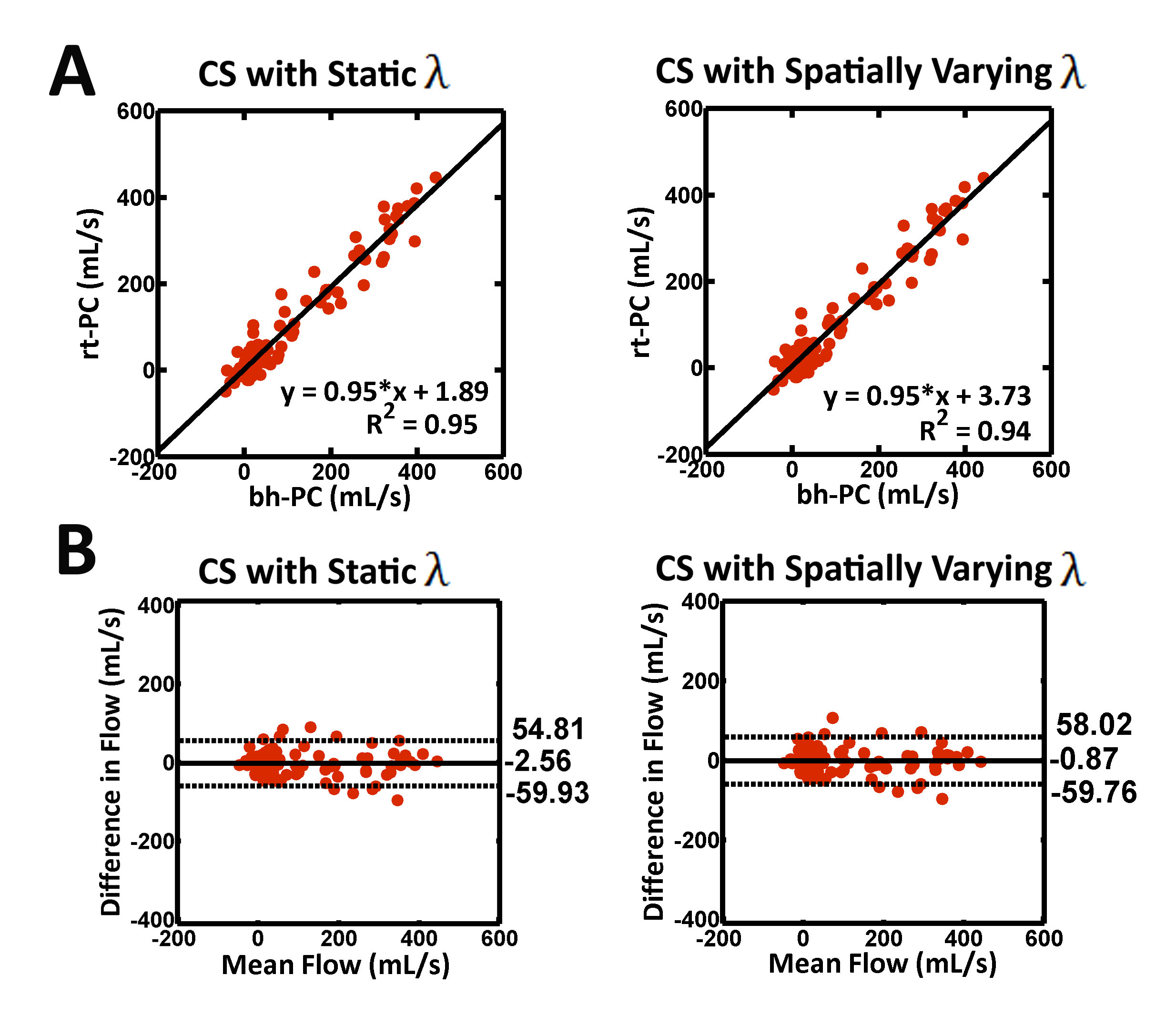
The mean artifact score for spatially varying λ was better (3.3 ± 0.8) than that for static λ (2.6 ± 0.5)(see Figure 2 for an example), where only the spatially varying λ was deemed clinical acceptable (score 3). Compared with clinical bh-PC, both static λ and spatially varying λ CS reconstructions produced flow values that were not significantly different (p>0.05). Figure 3 shows the scatter plots resulting from the Bland-Altman and linear regression analyses, which indicate that the flow values are strongly correlated and in good agreement between bh-PC and both CS reconstructions.

Conclusion

This study demonstrated a CS reconstruction method that uses spatially varying λ to reduce flickering artifacts arising from highly accelerated rt-PC MRI, without significant loss in accuracy. This reconstruction method produced relatively accurate flow metrics as compared with clinical bh-PC MRI. Future studies in a larger patient cohort are warranted to further evaluate the clinical utility.

Acknowledgements

NIH grant: R01HL116895, R01HL138578, R21EB024315, R21AG055954