3445

CArtesian sampling with Variable density and Adjustable temporal resolution (CAVA)

Adam Rich¹, Ning Jin², Yingmin Liu³, Lee C. Potter⁴, Orlando P. Simonetti^3,5,6, and Rizwan Ahmad^1,3

¹Department of Biomedical Engineering, The Ohio State University, Columbus, OH, United States, ²Siemens Medical Solutions, Columbus, OH, United States, ³Dorothy M. Davis Heart and Lung Research Institute, The Ohio State University, Columbus, OH, United States, ⁴Electrical and Computer Engineering, The Ohio State University, Columbus, OH, United States, ⁵Division of Cardiovascular Medicine, Department of Internal Medicine, The Ohio State University, Columbus, OH, United States, ⁶Department of Radiology, The Ohio State University, Columbus, OH, United States

Synopsis

We present a variable density Cartesian sampling method that allows retrospective adjustment of temporal resolution, providing added flexibility for real-time applications where optimal temporal resolution may not be known in advance. This method, called CArtesian sampling with Variable density and Adjustable temporal resolution (CAVA), is validated using real-time, free-breathing phase-contrast MRI data from four volunteers. Diagnostic quality images were successfully recovered at different temporal resolutions. Also, flow quantification based on CAVA was in good agreement with the breath-held segmented acquisition. In summary, CAVA provides a Cartesian alternative to Golden Angle-based radial sampling and can benefit a wide range of 2D real-time applications.

Purpose

For cardiac MRI (CMR), Cartesian sampling remains the most commonly employed acquisition strategy. However, for 2D real-time CMR with Cartesian sampling, temporal resolution must be selected in advance and cannot be changed post-acquisition. In contrast, Golden Angle-based radial acquisition allows altering temporal resolution retrospectively. This retrospective adjustment of temporal resolution provides added flexibility because optimal temporal resolution may not be known in advance. Although it is feasible to design a Cartesian sampling where phase-encoding increments between two consecutive readout lines are based on the Golden Ratio¹, such a strategy yields uniform sampling density and thus performs poorly at high acceleration rates. In this work, we propose a new Cartesian data sampling scheme, called CArtesian sampling with Variable density and Adjustable temporal resolution (CAVA). Distinguishing features of CAVA include (i) temporal resolution that can be adjusted retrospectively, (ii) variable density to preferentially sample the central k-space at higher rate, (iii) maintaining incoherence, and (iv) ensuring a fully sampled time average to facilitate sensitive map estimation. For validation, we utilized CAVA to collect phase-contrast MRI (PC-MRI) from four healthy volunteers and then reconstructed the images at six different temporal resolutions.

Methods

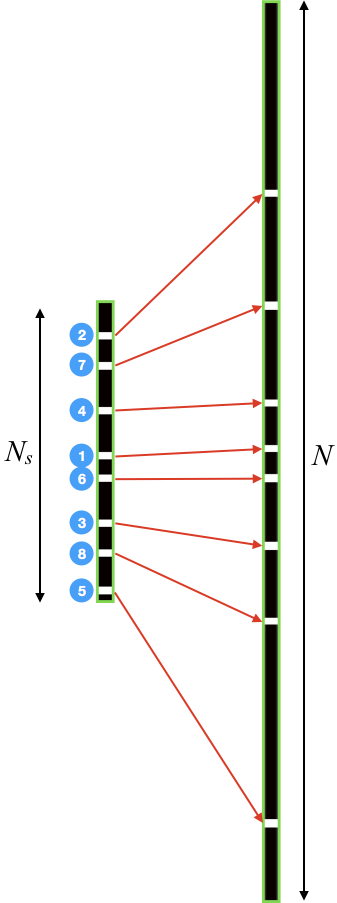
Generating CAVA - To distribute $$$M$$$ samples on a k_y-t Cartesian grid with $$$N_s$$$ phase-encoding (PE) lines, we first generate sampling on a smaller grid with $$$N_s$$$ PE lines $$$(N_s =\frac{N}{s},s>1)$$$. Starting from a randomly selected first PE index, $$$p_s(1)$$$, the index of the subsequent PE lines is sequentially advanced by $$$ gN_s$$$, yielding $$ p_s(i+1) =\left<p_s(i) + gN_s\right>_{N_s} \,\,\,\,\, \text{(Eq. 1)},$$ where $$$ p_s(i) $$$ is the PE index of the $$$i^{\text{th}}$$$ $$$ (i = 1,2,...,M)$$$, (sample on the grid with $$$N_s$$$ PE lines, $$$g$$$ is the golden ratio (0.618), and $$$\left<\cdot\right>_{N_s}$$$ represents modulo operation. Now the samples $$$ p_s(i) $$$ can be projected to a larger grid using a nonlinear stretching operation, yielding $$ p(i) = \left[ p_s(i) - k\,\text{sign}\left(\frac{N_s}{2}-p_s(i)\right) \left| \frac{N_s}{2}-p_s(i)\right|^{\alpha}+\frac{1}{2}(N-N_s)\right]\,\,\,\,\, \text{(Eq. 2)},$$ where $$$p(i)$$$ is the PE index of the $$$i^{\text{th}}$$$ sample on the grid with $$$N$$$ PE lines, $$$s$$$ controls the relative acceleration rate at the center of k-space compared to the overall acceleration rate, with $$$s>1$$$ ensuring that the sampling density is higher at the center of k-space, $$$\alpha\geq$$$ controls the transition from high-density central region to low-density outer region, $$$\left[\cdot\right]$$$ represents the rounding operation, and constant $$$k>0$$$ is selected such samples $$$p_s=1$$$ and $$$p_s=N_s$$$ are mapped to $$$p=1$$$ and $$$p=N$$$, respectively. In this work, we selected $$$s=3$$$ and $$$\alpha=3$$$.

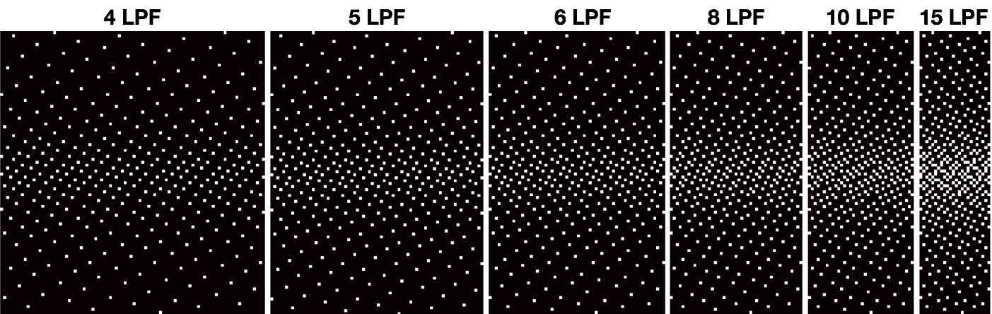
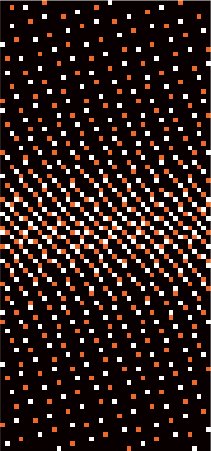
Figure 1 depicts the stretching process from smaller $$$N_s$$$-grid to the final $$$N$$$-grid. Figure 2 shows CAVA when the same sequence of $$$p$$$ values is binned with different lines per frame (LPF) values. Figure 3 shows two interleaved CAVA samplings for PC-MRI, where the prestretching offset between the two samplings was set at $$$gN_s/2$$$

Data Acquisition—For validation, data was collected from four volunteers on a 3T (Prima, Siemens Healthcare, Erlangen, Germany) using a gradient echo, through-plane flow quantification pulse sequence with TE = 2.12ms, TR = 4.1ms, flip angle = 15^o, spatial resolution 2.9x2.4 mm, acquisition matrix 84x128, and 10s of free breathing acquisition time.

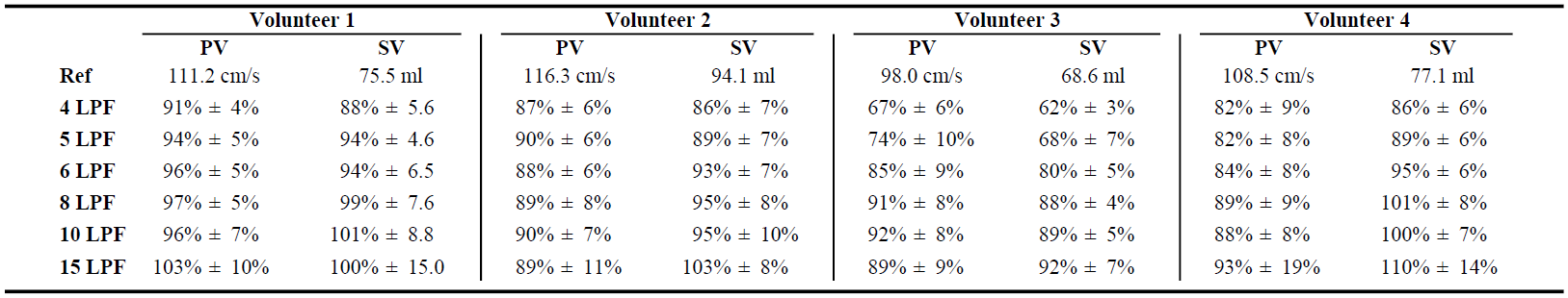
Image Recovery—Images were reconstructed using ReVEAL²at six different temporal resolutions: 4 LPF (33.0 ms), 5 LPF (41.2ms), 6 LPF (49.4ms), 8 LPF (65.9ms), 10 LPF (82.4ms) and 15 LPF (123.6ms) with net acceleration rate R = 21, 16.8, 14, 10.5, 8.4, 5.6 respectively. To obtain reference values, segmented acquisition was performed using a gradient echo, through-plane flow quantification sequence with TE = 2.53ms, TR = 4.63ms, temporal resolution 37.1ms, flip angle =15^o, and spatial resolution 2.1x2.1mm.

Image Analysis—All contours were drawn using freely available Segment software (Medviso, Lund Sweden). Peak velocity (PV) and stroke volume (SV) were computed for each heartbeat in the real time data and compared against values from the reference segmented acquisition.

Results and Discussion

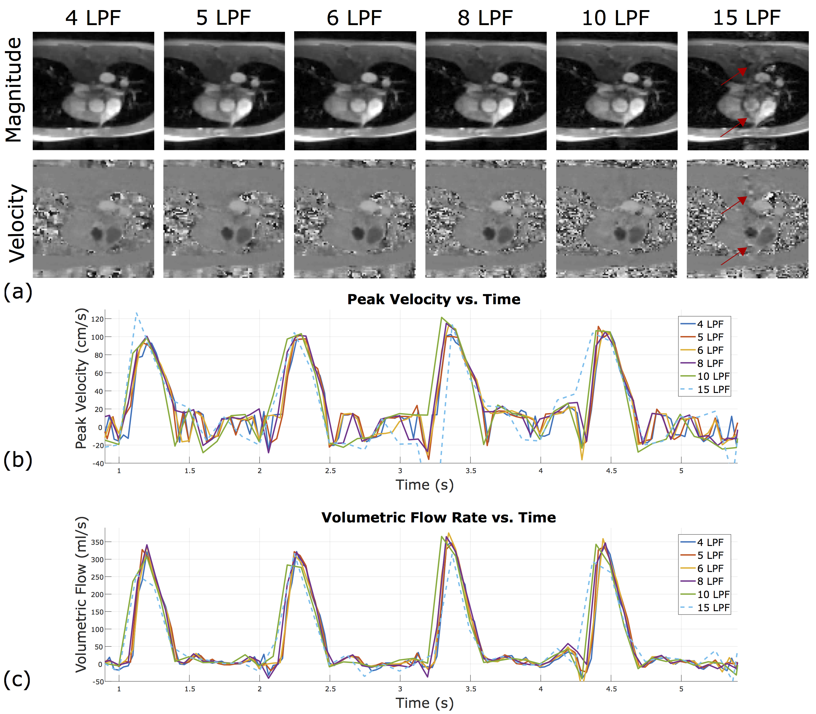
The results are summarized in Figure 4, and representative images are shown in Figure 5a. The spatial quality of the image is maintained across different LPF values, even at LPF=4. Visible image artifact was observed for LPF=15 due to model mismatch. Also, the velocity-time profiles (Figure 5b-c) were reproducible across different temporal resolution. Some underestimation of PV and SV was observed at LPF=4, perhaps due to over regularization, and temporal blurring was observed in LPF=10 and LPF=15.

Conclusion

We have proposed a new sampling method, CAVA, that exhibits variable density and adjustable temporal resolution. CAVA provides a Cartesian alternative to Golden Angle-based radial sampling and may benefit a wide range of dynamic MRI applications.

Acknowledgements

This work was partially funded by NIH grants R01HL135489 and R21EB021655.

References

[1] Guo L, Derbyshire JA, Herzka DA. Magnetic Resonance in Medicine 2015;76:417-429

[2] Rich A, Potter LC, Jin N, Ash J, Simonetti OP, Ahmad R. Magnetic Resonance in Medicine 2015;76:689-701

Figures

Figure 1: The stretching process employed in CAVA. First, a smaller grid is sampled with Golden Ratio jumps between consecutive samples (Eq. 1). Only eight samples and their acquisition order is shown. The samples are then projected to a larger (final) grid (Eq. 2), enabling variable density. Here, $$$N$$$=120 and $$$N_s$$$=40.

Figure 2: Retrospective adjustment of temporal resolution with CAVA. All sampling patterns were generated from the same sequence of phase coding index. The resolution was retrospectively changed by assigning different number of lines per frame (LPF). Here, $$$M=360$$$, $$$N=96$$$.

Figure 3: An example of CAVA for 2D PC-MRI. The composite sampling pattern is a union of two independent CAVA, with one used to collect compensated data and the other used to collect velocity encoded data. The two CAVA patterns consistently interleave each other because they are shifted with respect to each other before stretching. Here, LPF=8 and $$$N=96$$$.

FIgure 4: Tabulated values for PV and SV from four volunteers. The mean and standard deviation for all the heartbeats for a given LPF value are shown as a percentage of the reference value.

Figure 5: Data reconstructed using ReVEAL. (a) Selected frames from a single volunteer for LPF=4, 5, 6, 8, 10, 15. (b) Peak velocity profiles from different LPF values. (c) Volumetric flow rate from different LPF values.

Proc. Intl. Soc. Mag. Reson. Med. 26 (2018)

3445