3436

On the Influence of Intravoxel Velocity Distributions on the Noise of Phase Contrast Velocimetry

Simon Schmidt¹, Sebastian Flassbeck¹, Mark E. Ladd¹, and Sebastian Schmitter^1,2

¹Medical Physics in Radiology, German Cancer Research Center (DKFZ), Heidelberg, Germany, ²Physikalisch-Technische Bundesanstalt (PTB), Braunschweig and Berlin, Germany

Synopsis

In this work we investigate the influence of intravoxel velocity distributions on the velocity noise in phase contrast velocimetry. Intravoxel velocity distributions are directly measured via Fourier velocity encoding and subsequently fitted by Gaussian distributions. Taking intravoxel dephasing due to a finite distribution width into account, a noise-optimized VENC is calculated for phantom flow measurements and in-vivo data at 7 Tesla.

Purpose / Introduction

Phase-contrast MRI is a standard velocity imaging technique to noninvasively characterize hemodynamics in-vivo. The velocity is obtained by acquiring at least two images with different first gradient moments $$$m_1=\int_{t_0}^{t_{end}}G(t)\cdot t ~ dt$$$. Here $$$t_0$$$ is the isodelay time point (typically RF pulse center) and $$$t_{end}$$$ is the echo time. The corresponding velocity noise is commonly [1] described as $$$\sigma_v=\frac{\sqrt{2}~VENC}{\pi~SNR}$$$ with velocity sensitivity $$$VENC=\frac{\pi}{\gamma\mid\triangle{m_1}\mid}$$$, gyromagnetic ratio $$$\gamma$$$, signal-to-noise-ratio $$$SNR=\frac{S}{\sigma_S}$$$ and standard deviation of the magnitude noise $$$\sigma_S$$$. As the velocity noise is linearly depenent on $$$VENC$$$, low $$$VENC$$$ values are typically desirable and have led to increased popularity of multi-VENC methods [2-5].

This theory is based on the assumption that the velocity distribution within a voxel is a delta peak. Under real conditions, however, the velocity distribution can cover a broad spectrum. In this work the intravoxel velocity distribution is measured in a flow phantom and in-vivo and then used to model the velocity noise $$$\sigma_v$$$ as a function of $$$VENC$$$.

Theory

Given the velocity distribution $$$S(v)$$$ within a voxel, the signal can be calculated as $$$S=\int{S(v)}e^{i~v~\gamma~m_1}dv$$$ when applying a first gradient moment $$$m_1$$$ for velocity encoding (assuming $$$m_i=0~,~i\neq1$$$). According to Gaussian noise propagation the velocity noise for a phase-contrast acquisition is $$$\sigma_v=\sqrt{\frac{\sigma_S}{\mid\int{S(v)}e^{i~v~\gamma~m_1^1}dv\mid^2}+\frac{\sigma_S}{\mid\int{S(v)}e^{i~v~\gamma~m_1^2}dv\mid^2}}\cdot\frac{1}{\gamma\mid{m_1}^1-m_1^2\mid}$$$. In the special case of the frequently used symmetric encoding ($$$m_1^1=-m_1^2$$$), this can be simplified to $$$\sigma_v=\frac{\sqrt{2}\sigma_S.}{\gamma\mid{2}m_1^1\mid\cdot\mid\int{S(v)}e^{i~v~\gamma~m_1^1}dv\mid}$$$. Decreasing $$$m_1^1$$$ is often desired to reduce the velocity noise, but in fact it leads to two competing mechanisms: it decreases the velocity noise by $$$\frac{1}{\mid{2}m_1^1\mid}$$$ but also increases the velocity noise by $$$\frac{1}{\mid\int{S(v)}e^{i~v~\gamma~m_1^1}dv\mid}$$$. The latter term represents the loss of signal due to intravoxel dephasing. Therefore an optimal $$$m_1^1$$$ and corresponding $$$VENC_{opt}$$$ exists that minimizes the velocity noise.

Methods

Fourier velocity encoding (FVE) acquisitions to measure the intravoxel velocity distributions [6] were performed in a phantom and in-vivo at 7T (Siemens, Germany) using a 28-channel knee coil (Quality Electrodynamics, USA). An agarose-filled cylindrical phantom containing four water-filled pipes with diameters $$$4.2~/~7.8~/~12.1~/~15.5mm$$$ and water flowing through the two largest pipes was used. A programmable physiological flow pump (Shelly Medical Imaging Technologies, Canada) was used to create constant flow of different flow rates as well as a pulsatile flow profile. In-vivo data targeting the femoral artery of a healthy volunteer were acquired after obtaining consent to an IRB approved protocol.

The phantom and in-vivo FVE acquisitions were performed with cardiac triggering to allow the reconstruction of different cardiac phases. Resolution: $$$1mm\cdot{1}mm\cdot{1.5}\frac{cm}{s}$$$, FOV: $$$128mm\cdot{128}mm\cdot{168}\frac{cm}{s}$$$, TE: $$$14.2ms$$$. Gaussian distributions were fitted to the data in MATLAB (The Mathworks, USA), and subsequently $$$VENC_{opt}$$$ values were calculated. A standard 2D velocity sequence was acquired for both phantom and in-vivo experiments using $$$VENC=100\frac{cm}{s}$$$.

Results

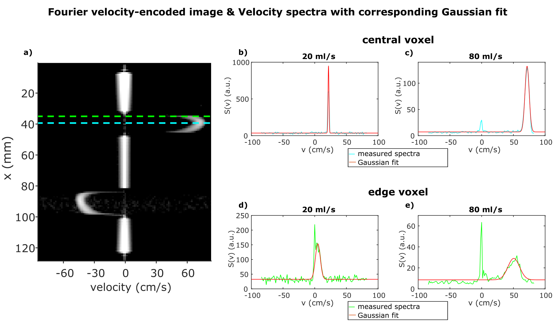
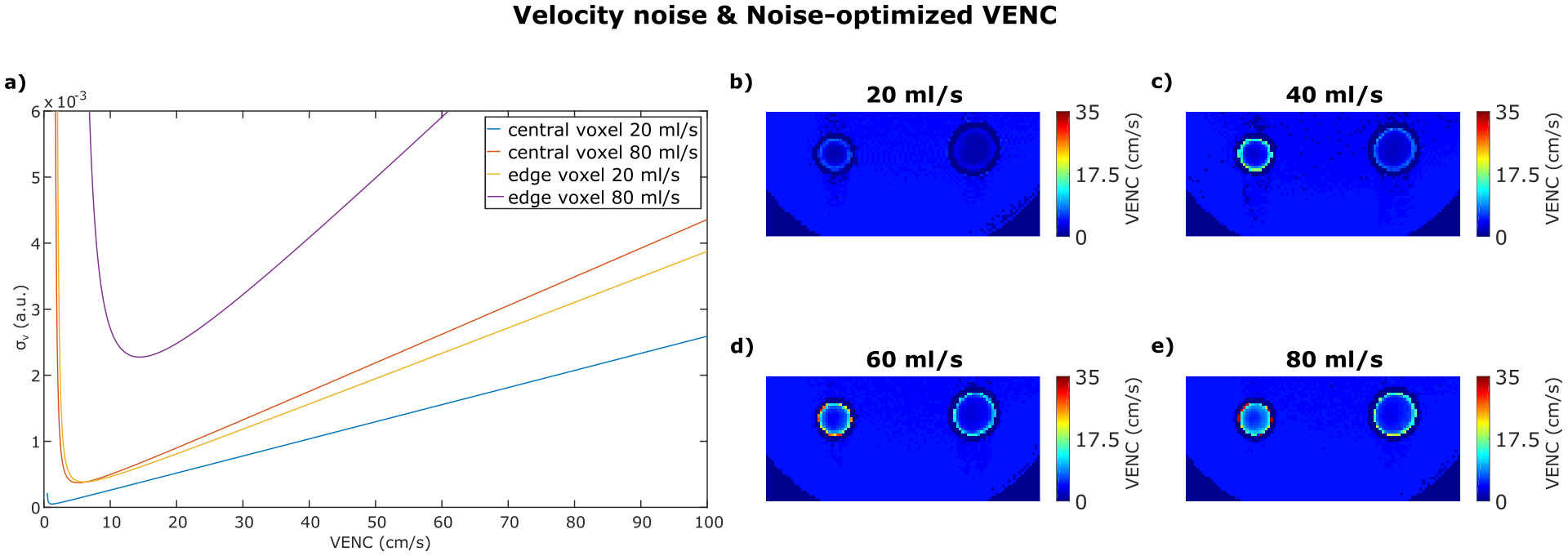
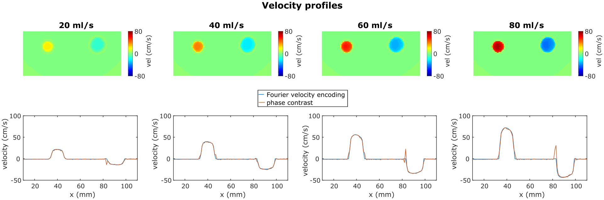
Figure 1 shows a FVE image and corresponding velocity spectra with fitted Gaussian distributions for different constant flow rates. The spectra show an additional peak at $$$v=0\frac{cm}{s}$$$ assumingly originating from static tissue which was neglected in further analysis. For constant flow, $$$VENC_{opt}$$$ increases with increasing flow rate and distance to the pipe center (Fig. 2). The man values of the Gaussian distributions agree with velocities measured by phase-contrast velocimetry (Fig. 3). In voxels with high spatial velocity gradients, $$$VENC_{opt}$$$ of up to $$$30\frac{cm}{s}$$$ are obtained for pulsatile flow in the phantom as well as in-vivo for the given imaging parameters. Note that if single-sided encoding ($$$m_1^1=\triangle{m_1},~m_1^2=0$$$) is used, $$$VENC_{opt}$$$ will double compared to the symmetric encoding used here.

Discussion

In this work we modeled the velocity noise as a function of $$$VENC$$$. The results demonstrate that simply lowering $$$VENC$$$, as assumed in Multi-VENC imaging, does not necessarily result in reduced velocity noise: for the in-vivo data we obtained $$$VENC_{opt}=30\frac{cm}{s}~(60\frac{cm}{s})$$$ in double- (single-) sided encoding close to the vessel wall.

Limitations of the FVE in-vivo study were i) the long echo-time leading to flow related displacement artifacts (slice and femoral artery were not perfectly orthogonal) and ii) the long scan time of $$$130min$$$ leading to degradation due to possible movement.

Our findings have, for example, implications for wall shear stress (WSS) imaging: WSS is derived from velocities close to the vessel wass, i.e. where we measured the highest $$$VENC_{opt}$$$, and WSS is particularly sensitive to noise due to the spatial derivative. Furthermore, we used a spatial resolution of $$$1mm\cdot{1}mm$$$, but if resolution is lowered to $$$2mm\cdot{2}mm$$$ (typical in aortic 4D flow MRI), $$$VENC_{opt}$$$ is assumed to increase to approximately $$$60\frac{cm}{s}~(120\frac{cm}{s})$$$ for double- (single-) sided encoding.

Furthermore the obtained results can be used to develop an optimized $$$m_1$$$ pattern for flow MR Fingerprinting [7].

Acknowledgements

No acknowledgement found.

References

[1] Lee, A. T., Bruce Pike, G. and Pelc, N. J. (1995), Three-Point Phase-Contrast Velocity Measurements with Increased Velocity-to-Noise Ratio. Magn. Reson. Med., 33: 122–126.

[2] Nett, E. J., Johnson, K. M., Frydrychowicz, A., Del Rio, A. M., Schrauben, E., Francois, C. J. and Wieben, O. (2012), Four-dimensional phase contrast MRI with accelerated dual velocity encoding. J. Magn. Reson. Imaging, 35: 1462–1471.

[3] Ha, H., Kim, G. B., Kweon, J., Kim, Y.-H., Kim, N., Yang, D. H. and Lee, S. J. (2016), Multi-VENC acquisition of four-dimensional phase-contrast MRI to improve precision of velocity field measurement. Magn. Reson. Med., 75: 1909–1919.

[4] Callaghan, F. M., Kozor, R., Sherrah, A. G., Vallely, M., Celermajer, D., Figtree, G. A. and Grieve, S. M. (2016), Use of multi-velocity encoding 4D flow MRI to improve quantification of flow patterns in the aorta. J. Magn. Reson. Imaging, 43: 352–363.

[5] Schnell, S., Ansari, S. A., Wu, C., Garcia, J., Murphy, I. G., Rahman, O. A., Rahsepar, A. A., Aristova, M., Collins, J. D., Carr, J. C. and Markl, M. (2017), Accelerated dual-venc 4D flow MRI for neurovascular applications. J. Magn. Reson. Imaging, 46: 102–114.

[6] Moran, P. R. 1982. A flow velocity zeugmatographic interlace for NMR imaging in humans. Magn. Reson. Imaging 1: 197-203.

[7] Flassbeck, S., Schmidt, S., Breithaupt, M., Bachert, P., Ladd, M. E., Schmitter, S., Quantification of Flow by Magnetic Resonance Fingerprinting. In Proceedings of the 25th Annual Meeting of the ISMRM, Honolulu, HI, USA, 2017. Abstract 0128.

Figures

Figure 1: a) Fourier velocity-encoded image with a resolution of 1.5 cm/s in the velocity direction from a phantom measurement. b)-e) show corresponding velocity spectra for different constant pump rates. a) and b) correspond to a voxel located in the middle of the smaller tube (blue dashed line) while c) and d) show the spectrum of a voxel at the edge of the tube (green dashed line). With increasing pump rate, the distribution slightly broadens for the central voxel. At the edge of the tube the corresponding spectra are significantly broadened already at low pump rates, which further increases with high pump rates.

Figure 2: a) Velocity noise as a function of VENC for a central and edge voxel for the lowest and highest constant pump setting. With increasing width of the spectra, the minimal noise increases as well as the corresponding optimal VENC. b)-e) Noise-optimized VENC maps for different constant pump rates. Corresponding velocity profiles through the smaller tube can be seen in Figure 3. At the edge of the tubes the velocity spectra are broader due to the high spatial variation of the velocity profile, resulting in higher optimal VENC values of up to 30 cm/s for symmetric encoding (60 cm/s for single-sided encoding).

Figure 3: Top row: Velocity maps obtained from the mean of the Gaussian fit for different constant pump settings. Bottom row: Comparison of the velocity profile obtained from Fourier velocity encoding and conventional phase contrast velocimetry along the black dashed lines in the top row. Given a Gaussian velocity distribution, the mean of the distribution is equivalent to the value obtained by phase-contrast velocimetry.

Figure 4 (animated): Noise-optimized VENC map for a phantom measurement and a pulsatile pump setting with corresponding mean velocity map and temporal velocity profile in the smaller tube. For comparison, the temporal velocity profile was also measured using phase-contrast velocimetry. For this setting the central voxels show elevated optimal VENC values compared to constant pump settings, but again edge voxels show the largest values of up to 30 cm/s.

Figure 5 (animated): In-vivo data targeting the femoral artery of a healthy volunteer. The noise-optimized VENC map with corresponding mean velocity map and temporal velocity profile are shown. For comparison, the temporal velocity profile was also measured using phase-contrast velocimetry. Optimal VENC values of up to 30 cm/s comparable to the pulsatile pump setting are observed.

Proc. Intl. Soc. Mag. Reson. Med. 26 (2018)

3436