3435
Exploring vessel inward normal computation for 4D flow based wall shear stress estimation in complex vessel geometries.1Department of Computer Science, Technical University of Munich, Munich, Germany, 2Department of Pediatric Cardiology and Congenital Heart Defects, German Heart Center Munich, Munich, Germany, 3Fraunhofer MEVIS Institute for Medical Image Computing, Bremen, Germany, 4Departments of Radiology and Biomedical Engineering, Northwestern University Feinberg School of Medicine, Chicago, IL, United States, 5Institute for Computational and Imaging Science in Cardiovascular Medicine, Charité Universitätsmedizin Berlin, Berlin, Germany
Synopsis
Wall shear stress (WSS) is a hemodynamic parameter which can be estimated from 4D flow MRI. The aim of this work was to advance the surface inward normal computation for complex (i.e. cone-shaped) vessel geometries and thus to improve the accuracy of wall shear stress estimates. We propose a Gauss gradient field approach to adapt to complex vessel courses and evaluate our method using synthetic flow data and selected patient data. Results show that correct inward normal definition is crucial for reliable WSS estimates, in particular in cases where complex vessel geometries are present.
Introduction
4D flow MRI allows the image-based estimation of quantitative wall shear stress (WSS) in vascular structures. WSS ($$$\vec{\tau}$$$) at any vessel wall point is defined as $$\vec{\tau}=2\eta\dot{\epsilon}\cdot\vec{n}$$ with $$$\vec{n}$$$ = vessel surface inward normal, $$$\eta$$$ = dynamic viscosity, and $$$\dot{\epsilon}$$$ = velocity deformation tensor. Furthermore, the oscillatory shear index (OSI) is defined as: $$OSI=\frac{1}{2}\left(1-\frac{|\int_{0}^{T}\vec{\tau}\cdot dt| }{\int_{0}^{T}|\vec{\tau}|\cdot dt}\right)$$ Previous works studied the impact of MRI acquisition parameters on WSS estimates1 though the burden of inaccurate inward normal definition is unknown. Most commonly, WSS and OSI are estimated by analyzing reformatted 2D planes2-4 and the inward normal at each wall point is only comprised of the vector component lying on the respective plane. However, in case of complex vessel geometries (e.g. stenosis, dilatation) the inward normal may deviate from the analysis plane.The aim of this work was to (1) introduce a method to accurately compute surface inward normals in cone-shaped vessel regions given the typical 4D flow MRI image data, and to (2) study the systematic error of WSS/OSI estimates when only the inplane inward normal component is considered.
Methods
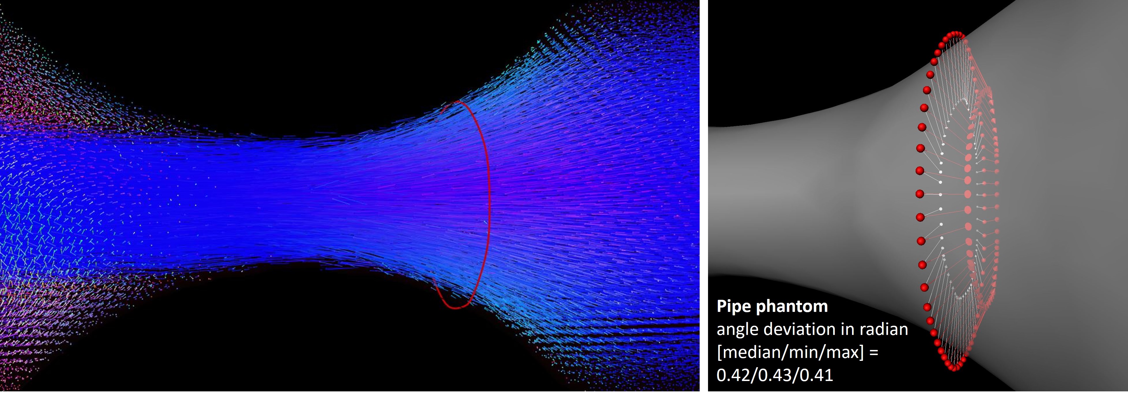
Synthetic data. Steady flow was simulated through a pipe with narrowing on a high resolution grid (fig. 1) using Comsol Multiphysics (resolution = 0.7x0.7x0.7 mm3; min/max vessel diameter = 10.3/33.5 mm; mean velocity at inlet = 3.89 cm/s).
In-vivo data. Six 4D flow MRI data sets of patients with stenotic or dilated vessel geometry were included. Scans were performed on a 1.5T Avanto (N=3) or 3T Trio (N=3) system with: TE/TR = 2.6/5.1 ms; FOV ~ 400x300x60 mm3; voxel dimension = 1.7-2.5 x 1.7-2.5 x 2.0-2.5 mm3; VENC = 150-300 cm/s; parallel imaging with R = 5; prospective ECG triggering covering the full cycle; navigator gating. Data pre-processing included phase offset correction (via polynomial function fitting), background noise masking, and automatic phase unwrapping if needed.
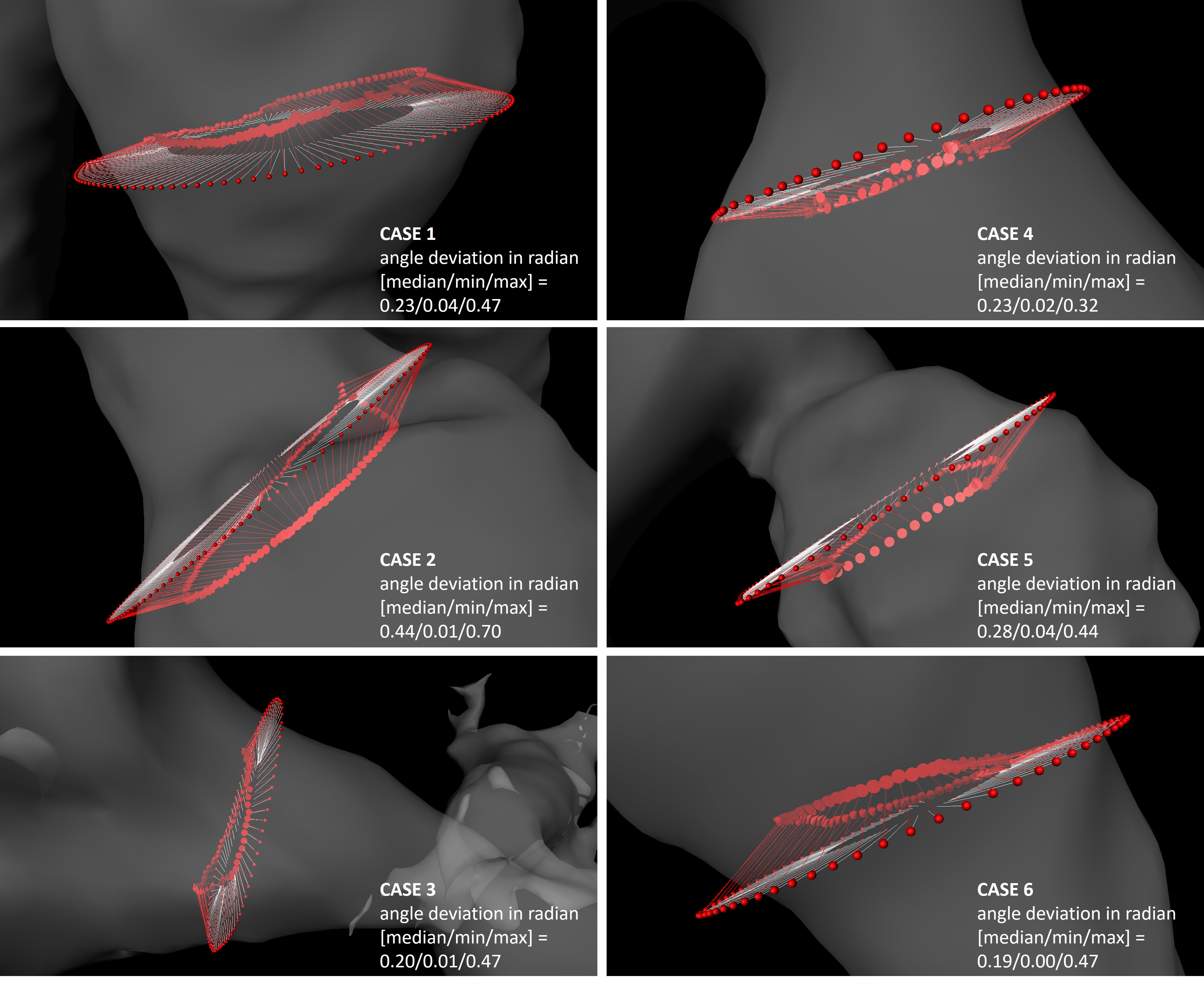
WSS computation. Vessels were segmented from the generated PC-MRA image using a watershed-based algorithm. For each case, one analysis plane was placed in the dilated/stenotic vessel region and vessel contours were tracked through all time frames (fig. 2). The binary vessel mask was used to derive a Gauss gradient field ($$$\boldsymbol{G}$$$) to advance the computation of the vessel inward normal at each sampled contour point $$$\boldsymbol{x}$$$: $$\vec{n}_\boldsymbol{x}=\vec{a}_\boldsymbol{x}+\vec{g}_{\boldsymbol{x},p}$$ where $$$\vec{g}_{\boldsymbol{x},p}=\left(\boldsymbol{G}_\boldsymbol{x}\cdot\vec{p}\right)\vec{p}$$$ is the projection of $$$\boldsymbol{G}_\boldsymbol{x}$$$ (local Gauss gradient vector) onto the unit plane normal $$$\vec{p}$$$, and $$$\vec{a}_\boldsymbol{x}$$$ is the conventional inward normal lying on the analysis plane. WSS was then estimated at each contour point using a B-spline image function based approach5 with η = 0.0032 Pa s. Regarding synthetic data, we analyzed single timepoint WSS (WSSsingle); regarding in-vivo data, we analyzed WSS at peak velocity (WSSpeak) and OSI. Estimates were binned into twelve angular segments to compute mean±STD per segment. All image analysis was implemented using the MevisLab6 framework.
Evaluation. WSSsingle, WSSpeak, and OSI were assessed segment-wise regarding absolute and relative differences of estimates based on conventional vs. adapted inward normal. Angle deviations between conventional ($$$\vec{a}_\boldsymbol{x}$$$) and adapted ($$$\vec{n}_\boldsymbol{x}$$$) inward normals were computed.
Results
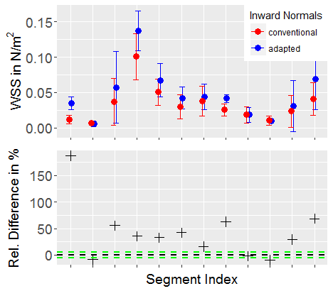
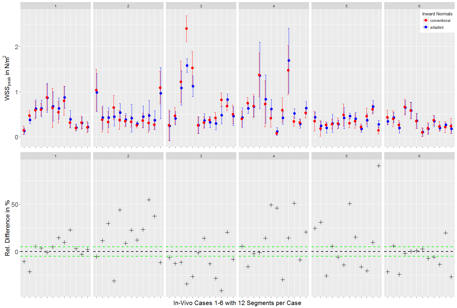
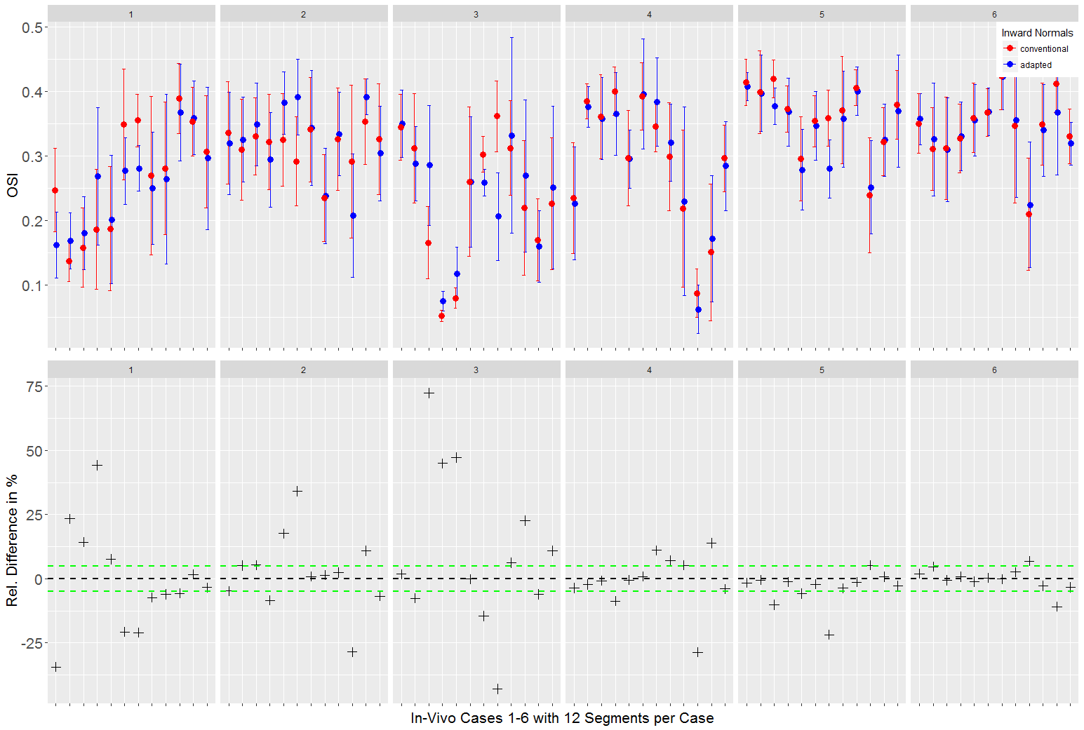
Both synthetic and in-vivo data results show noticeably deviated inward normals when the Gauss gradient field is incorporated (fig. 1, 2) with angle deviations ranging from 0.00-0.70 rad for in-vivo data and 0.41-0.43 rad for the pipe phantom. With adapted inward normals, synthetic data results show an increase in WSSsingle by 45.9±49.6% (fig. 3). Regarding in-vivo data results, we observe differences in WSSpeak of 8.5±7.5%, 24.4±15.5%, 18.1±12.1%, 21.6±18.2%, 25.8±23.9%, and 10.9±9.7% (fig. 4), and in OSI of 15.8±13.3%, 10.5±10.8%, 23.1±23.2%, 7.2±8.0%, 4.6±6.0%, and 3.0±3.2% for cases 1-6, respectively (fig. 5). All numbers indicated above are given as mean±STD over all twelve segments.Discussion
Synthetic data results show a clear underestimation when inward normal vectors are not adapted to the local vessel geometry. Here, an outlier is present due to a very subtle flow profile and thus comparably small WSSsingle values, which challenges the assessment in terms of relative differences. Synthetic data should be optimized to better represent flow velocities as given in the in-vivo data. In-vivo data results clearly show that adapted inward normal vectors result in strong deviations of WSSpeak and OSI, which should not be neglected when using these parameters in a clinical study. Particularly, differences are very pronounced for high angular deviations. Concering limitations, this study did not assess differences in WSS/OSI contour-point-wise (only segment-wise) and thus did not correlate each contour point WSS/OSI value with the angular deviation of the conventional and adapted inward normal at this point.Conclusion
The proposed method may be used to more precisely define vessel inward normal vectors for increased WSS and OSI estimation. Particularly, this is crucial where the vessel wall depicts a cone-shaped course.Acknowledgements
This project is funded by Deutsche Herzstiftung e.V., Frankfurt a. M., Germany.References
[1] S. Petersson et al., “Assessment of the accuracy of MRI wall shear stress estimation using numerical simulations,” J Magn Reson Imaging, vol. 36, no. 1, pp. 128–138, 2012. [2] M. Markl et al., “In vivo wall shear stress distribution in the carotid artery: effect of bifurcation geometry, internal carotid artery stenosis, and recanalization therapy,” Circ Cardiovasc Imaging, vol. 3, no. 6, pp. 647–655, 2010. [3] A. J. Barker et al., “Bicuspid Aortic Valve Is Associated With Altered Wall Shear Stress in the Ascending Aorta,” Circ Cardiovasc Imaging, vol. 5, no. 4, pp. 457–466, 2012. [4] M. D. Hope et al., “MRI hemodynamic markers of progressive bicuspid aortic valve-related aortic disease,” J Magn Reson Imaging, vol. 40, no. 1, pp. 140–145, 2014. [5] A. F. Stalder et al., “Quantitative 2D and 3D phase contrast MRI: Optimized analysis of blood flow and vessel wall parameters,” Magn Reson Med, vol. 60, no. 5, pp. 1218–1231, 2008. [6] F. Ritter et al., “Medical image analysis,” IEEE Pulse, vol. 2, no. 6, pp. 60–70, 2011.Figures