3402

Extending the small tip angle approximation to the non-equilibrium initial condition

Bahman Tahayori^1,2,3, Zhaolin Chen², Gary Egan², and N. Jon Shah ⁴

¹Electrical and Computer Systems Engineering, Monash University, Clayton, Australia, ²Monash Biomedical Imaging, Monash University, Clayton, Australia, ³Medical Physics and Biomedical Engineering Department, Shiraz University of Medical Sciences, Shiraz, Iran (Islamic Republic of), ⁴Department of Neurology, JARA, RWTH Aachen University, Aachen, Germany

Synopsis

We have applied Volterra series expansion to the Bloch equation and have calculated the kernels for an arbitrary initial condition. We have shown that small tip angle approximation can be extended to the non-equilibrium initial condition. Simulation results illustrated the validity of the extended small tip angle approximation.

Introduction

Small Tip Angle (STA) approximation has been widely used in Magnetic Resonance Imaging (MRI) literature to design non-adiabatic slice selective pulses [1-3]. The two key assumptions in STA are thermal equilibrium initial condition and stationary longitudinal magnetisation during the excitation [1-3]. We have extended STA to the non-equilibrium initial condition by expanding the Bloch equation using the Volterra series representation of non-linear dynamical systems. Theoretical as well as simulation results demonstrate that STA approximation can be used to design slice selective pulses even when the bulk magnetisation is not initially at equilibrium.

Methods

A linear system can be described completely by its impulse response. Volterra series extends the impulse response to nonlinear systems through an infinite sum of higher order convolution integrals using Volterra kernels [4,5]. Bilinear systems have convergent Volterra series expansion and the Volterra kernels can be calculated using matrix exponentials [5]. The Bloch equation, neglecting the relaxation effects, when the excitation is applied in the $x$ -direction is written as

$\dot{ \textbf{M}}= \left[\begin{array}{c}\dot{M}_{x'}\\\dot{M}_{y'}\\\dot{M}_{z'} \end{array}\right] = \left[ \begin{array}{ccc} 0& \Delta \omega & 0 \\ -\Delta \omega & 0 & \omega_{1}(t) \\ 0 & -\omega_{1}(t) & 0 \end{array} \right] \left[\begin{array}{c} {M}_{x'}\\{M}_{y'}\\{M}_{z'} \end{array}\right],$

where $\dot{ \textbf{M}}$ is the magnetisation vector, $\omega_1$ is the excitation and $\Delta\omega$ represents the off-resonance frequencies that can be generated by gradient fields. Assuming the magnetisation is initially at $\textbf{M}^0 = [M_x^0 \quad M_y^0 \quad M_z^0]^T$ , the zeroth and the first kernels for the Bloch equation are

$h_0 (t) = \left(\begin{array}{c} {M_x^0}\, \cos\!\left(\Delta{}\omega{}\, t\right) +{M_y^0}\, \sin\!\left(\Delta{}\omega{}\, t\right)\\ {M_y^0}\, \cos\!\left(\Delta{}\omega{}\, t\right) - {M_x^0}\, \sin\!\left(\Delta{}\omega{}\, t\right)\\ {M_z^0} \end{array}\right),$

$h_1 (t,\tau_1)= \left(\begin{array}{c} {M_z^0}\, \sin\!\left(\Delta{}\omega{}\, \left(t - {\tau{}}_{1} \right)\right)\\ {M_z^0}\, \cos\!\left(\Delta{}\omega{}\, \left(t-{\tau{}}_{1} \right)\right)\\ {M_x^0}\, \sin\!\left(\Delta{}\omega{}\, {\tau{}}_{1}\right) - {M_y^0}\, \cos\!\left(\Delta{}\omega{}\, {\tau{}}_{1}\right) \end{array}\right).$

Theoretical Results

For the thermal equilibrium initial condition, the Volterra series expansion clearly shows that

$M_{xy} \triangleq M_x+ j M_y$ is the Fourier transform of the excitation

$k$ -space trajectory proportional to

$\omega_1$ [1]. When

$M_{xy}^0\neq 0$ , the Volterra series expansion shows that

$M_z$ is a combination of Fourier sine, Fourier cosine and Fourier transform of the excitation trajectory weighted by

$M_x^0$ ,

$M_y^0$ and

$M_z^0$ , respectively. For special cases when

$\textbf{M}^0 = [ 0 \quad M_0 \quad 0]^T$ and

$\textbf{M}^0 = [ M_0\quad 0 \quad 0]^T$ , where

$M_0$ is the thermal equilibrium, the

$M_z$ profile at the end of the pulse duration,

$t = \tau_p$ , is the Fourier sine and the negative Fourier cosine transform of the excitation pattern, respectively.

Simulation Results

To illustrate the validity of the theoretical results, we compared the approximation with the numerical solution of the Bloch equation for the following cases

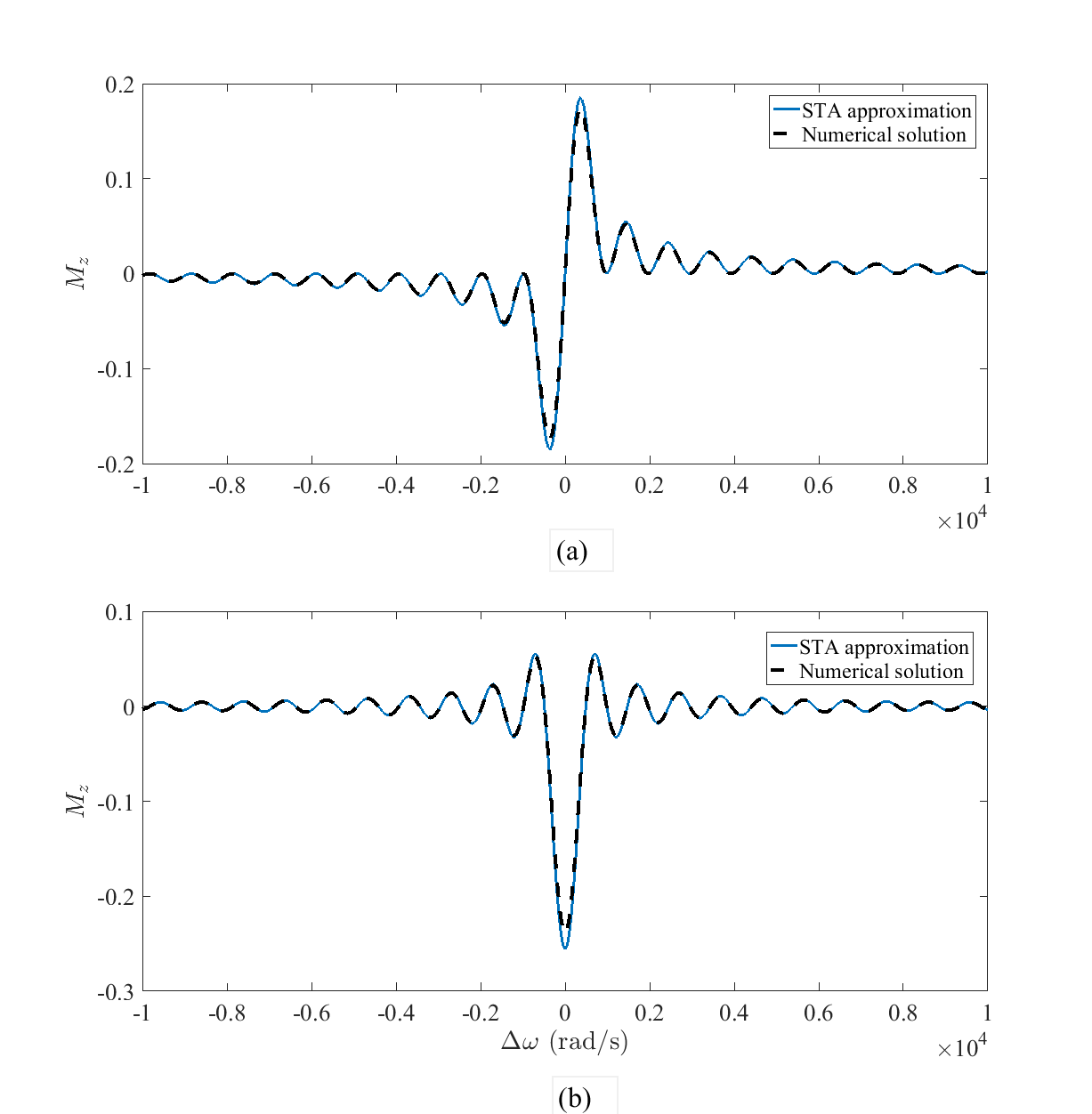
Forward problem: For a rectangular pulse excitation, we have calculated the $M_z$ profile when $\textbf{M}^0 = [ 1 \quad 0 \quad 0]^T$ and $\textbf{M}^0 = [ 0 \quad 1\quad 0]^T$ . The resultant $M_z$ profiles for the above initial conditions using the Volterra series kernels are

$M_z(\Delta\omega, \tau_p) = \mathcal{F}_s\{\omega_1(t)\} = \frac{\omega_1(1-\cos \Delta\omega\tau_p)}{\Delta\omega},$

and

$M_z(\Delta\omega, \tau_p) = \mathcal{F}_c\{\omega_1(t)\} = -\frac{\omega_1 \sin \Delta\omega\tau_p}{\Delta\omega},$

repectively. In the above equations, $\omega_1$ is the pulse amplitude and $\mathcal{F}_s$ and $\mathcal{F}_c$ are Fourier sine and cosine transforms, respectively. The numerical solution of the Bloch equation as well as the presented approximate solutions are shown in Figure 1. These results show that the approximate solution is in agreement with the numerical solution.

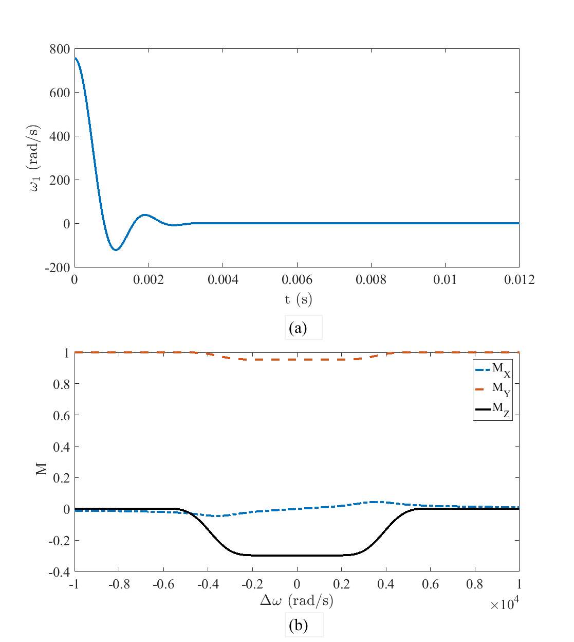
Backward problem: Assuming the magnetisation is initially at $\textbf{M}^0 = [ 0 \quad 1\quad 0]^T$ , we designed a slice selective pulse to rotate the magnetisation for $\pi/6$ about the $x$ -axis. Given that the Fourier cosine transform of a rectangular function is a half a sinc function, the excitation that tips the bulk magnetisation from the $+y$ -axis is a truncated half a sinc. The excitation pattern, as well as the resultant magnetisation profile are represented in Figure 2. Similar to the conventional Fourier method, to obtain a refocused slice, the gradient was reversed for half the time of the pulse duration with the same magnitude.

Conclusions

Here, we provided an alternative approach to address STA approximation using Volterra series expansion. Besides providing an insight into the validity of STA and how it works, we used this approach to extend the STA approximation to the non-equilibrium condition. We specifically looked at the cases where the magnetisation is initially aligned with

$x$ or

$y$ -axes and showed that the resultant profile in the

$z$ -direction simplifies to Fourier sine and cosine transforms, respectively. The results can be used to design pulses with more efficient slice selectivity, especially for inversion and refocusing pulses.

Acknowledgements

No acknowledgement found.

References

1. J. Pauly, D. Nishimura, and A. Macovski, "A k-space analysis of Small-tip-angle excitation," Magnetic Resonance in Medicine, vol. 81, pp. 43-56, 1989.

2. D. Nishimura, Principles of Magnetic Resonance Imaging, Stanford University, 1996.

3. M. Bernstein, K. King, and X. Zhou, Handbook of MRI pulse sequences, Elsevier, 2004.

4. L. Carassale and A. Kareem, "Modeling nonlinear systems by Volterra series," Journal of Engineering Mechanics, vol. 136, 2010.

5. R. Brockett, "The early days of geometric nonlinear control," Automatica, vol. 50, pp. 2203-2224, 2014.

Figures

Figure 1.

$M_z$ profile generated by a rectangular pulse excitation of a 12.8ms duration, (a) when the initial magnetisation was at

$[1\quad 0 \quad 0]^T$ and (b)

$[0 \quad 1 \quad 0 ]^T$ . The STA approximation solution is represented by the solid line and the numerical solution of the Bloch equation at the end of the pulse duration is shown by the dashed line.

Figure 2. (a) The designed pulse to tip the bulk magetisation from

$[0 \quad 1 \quad 0 ]^T$ for

$\pi/6$ and (b) the resultant slice profile. The gradient was switched on post excitation in the reverse direction to achieve a refocused slice.

Proc. Intl. Soc. Mag. Reson. Med. 26 (2018)

3402