Synopsis

Developing fast accurate large-tip-angle radiofrequency pulses and gradient trajectories suitable for ‘online’ use is a challenging problem. In this work we propose a novel method for the sub-second design of RF pulses and gradient trajectories through use of a suitably trained artificial neural network which attempts to learn the required pulse and gradient spoke parameters from B₁⁺ field spatial variations. A method for synthesising a large training database is also described. Our initial results highlight some of the challenges of this approach but suggest areas for future development.

Introduction

At high-field the electromagnetic field distribution becomes inhomogeneous and is highly variable with patient size. Improved uniformity can be achieved for slice-selective excitation through use of spokes^1,2; a series of subpulses played-out at different points in k-space. Design of parallel transmit Spokes pulses is complicated further at large-tip-angle due to the inherent nonlinear response of the Bloch equation and additional power and SAR constraints. Existing approaches trade-off target magnetisation accuracy with increased computational time^3-8. Developing fast accurate optimisation methods is a major effort to allow ‘online’ pulse and gradient design.

Previous work⁹ trained a network to design single-channel NMR spectroscopic radiofrequency pulses. In this work we propose a novel method for the sub-second design of RF pulses and gradient trajectories through use of a suitably trained artificial neural network which attempts to learn the required pulse and gradient spoke parameters from B₁⁺ field spatial variations.

Method

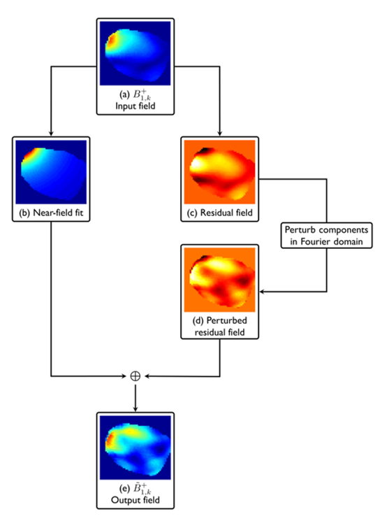
To learn the spatial variations of the B₁⁺ channel fields a training set of 60,000 x 8 B₁⁺ maps and optimal solutions was created (see Figure 1). From an initial full electromagnetic field simulation (provided by Nova Medical Inc., Wilmington, USA) of a male human head (downsampled to 25 x 25 voxels) within an 8-channel transmit/32-channel receive coil, individual transmit channel fields were fitted using a near-field dipole approximation over spatial coordinates. Subtraction of these fields resulted in a residual field which was decomposed into its Fourier components. The top 80% of Fourier coefficients were then randomly perturbed 60,000 times according to a normal distribution (0.1 variance) for each of the transmit channels.

Joint optimisation of 5-spoke RF pulses (amplitude and phase) plus gradient trajectory for slice inversion was performed for each of the entries within the B₁⁺ map database, using an optimal control approach with power regularisation (for implementation see³), yielding a set of 90 design parameters (5 x 8 channel amplitude, 5 x 8 channel phases, 5 x 2 k-space locations) for each B₁⁺ map set.

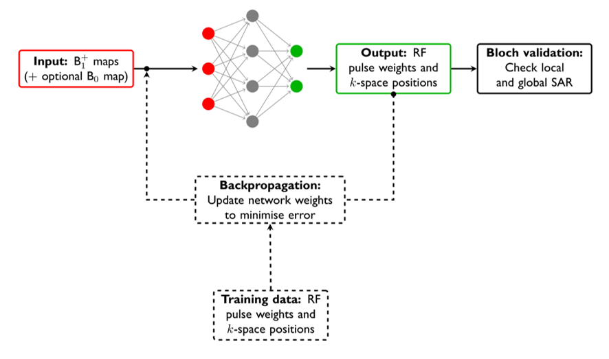
A neural network consisting of an input layer (2056 nodes), hidden layer (1000 nodes) with sigmoidal activation functions, and output layer (90 nodes) was employed. The network weights were iteratively updated using a commercial backpropagation algorithm with conjugate gradient descent (MATLAB, Natwick, USA) to minimise the squared error between the neural network outputs and training design parameters (see Figure 2). The training data was feature scaled and randomly divided towards 70% training, 30% validation.

Results

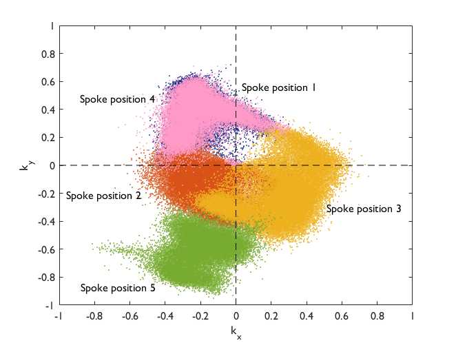
Creation of the training data (B₁⁺ maps and optimal solutions) took 14 hours to compute using a high-performance computing facility (3 x 16 processors, 2.66 GHz). The optimised k-space 5-spoke locations (see Figure 3) are shown to be distributed in clusters. During the training phase, the number of hidden nodes was adjusted to achieve a balance between training error, cross-validation error and overall training time (18 hours), resulting in a hidden layer of size 1000.

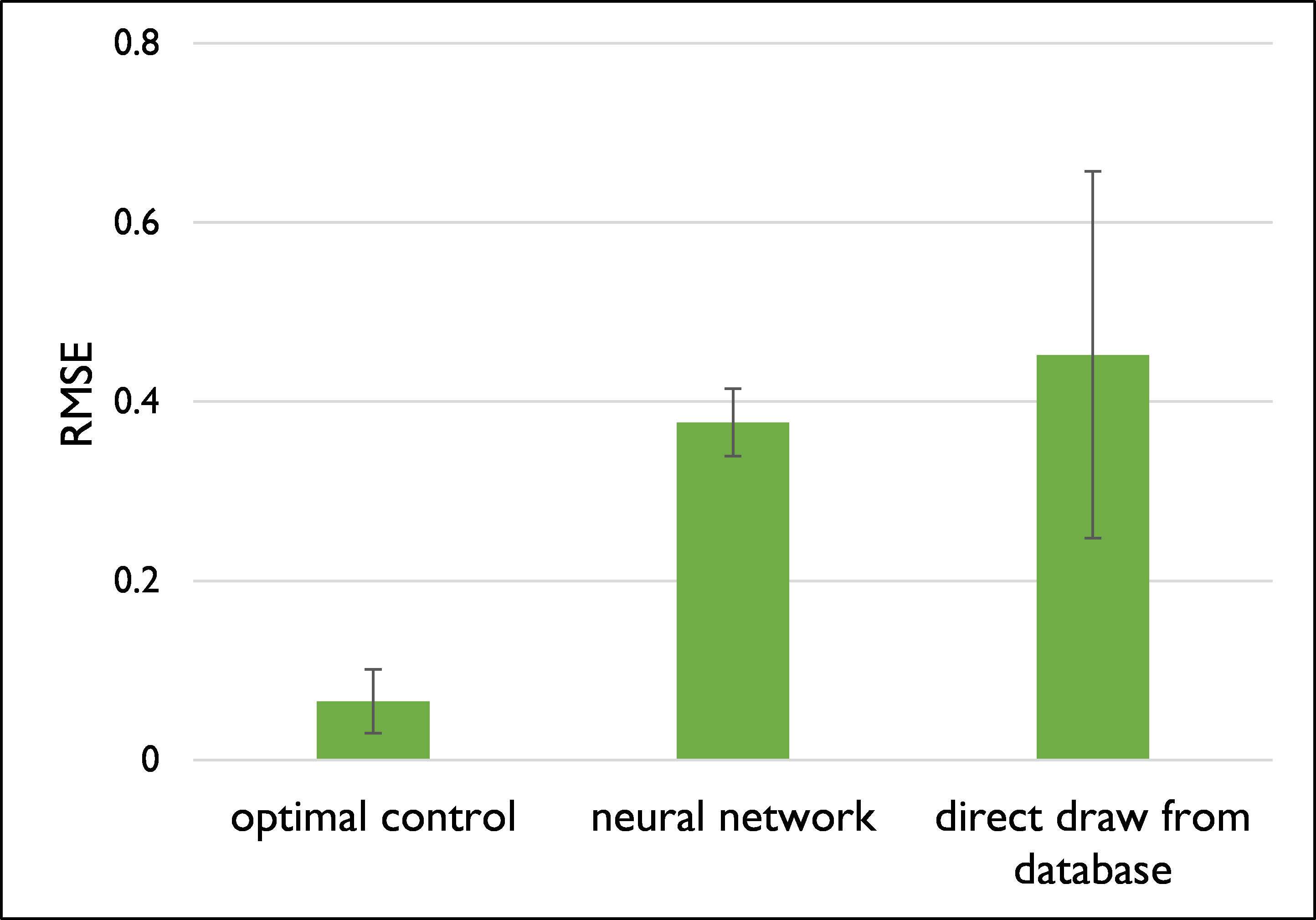
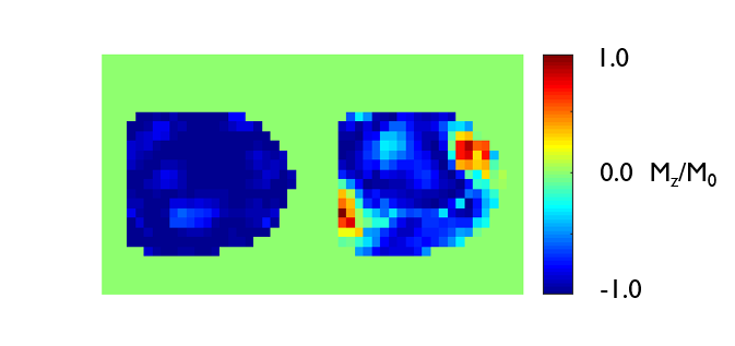
On an unseen set of 10 B₁⁺ maps, the network achieved a root-mean-square error (RMSE) of 0.38±0.04, with an average design time of 0.1 seconds (desktop PC, 3.70 GHz processor). In comparison, applying the full optimal control method achieved a substantially lower 0.06±0.04 RMSE with an average optimisation time of 370 seconds. Drawing a set of parameters directly from the training data yielded a 0.45±0.20 RMSE.

Discussion

We have proposed a new method for the sub-second design of large-tip-angle parallel transmit pulses based on learning the spatial variations within patient field maps. Our initial results show inferior inversion performance as compared to joint-optimisation of Spokes pulses using a full optimal control. We only observe a slight improvement over drawing parameters directly from the training set, suggesting our network design is heavily biased and not able to fully regress the 90 design parameters from the given field maps.

A likely factor in this can be found in Figure 3, demonstrating that the 5-spoke k-space locations for each of the training set entries are located in clusters. This reflects the small perturbation model that was used to create the training data and the down-sampling that was required to reduce the computation time required to create a large database. A potential for future work will be to apply our approach to inversion pulse design for the abdomen – where the degree of B₁⁺ field variation between patients is greater. In addition, increasing the number of nodes and hidden layers in the model will reduce biasing but would require a larger training set to prevent over-fitting.

Acknowledgements

References

[1] Saekho S. et al. (2005): MRM. 53: 479-484

[2] Saekho S. et al. (2006): MRM. 55: 719-724

[3] Cao Z. et al. (2016): MRM. 75: 1198-1208

[4] Xu D. et al. (2008): MRM. 59: 547-560

[5] Grissom W. et al. (2008): MRM. 59: 779-787

[6] Grissom W. et al. (2009): IEEE Trans Med Imaging. 28: 1548-1559

[7] Setsompop K. et al. (2008): MRM. 195: 76-84

[8] Gras V. et al. (2016): JMR. 261: 181-189

[9] Gezelter J. et al. (1990): JMR. 90: 397-404