3382
Optimal Regularization Parameter Selection for Constrained Reconstruction Using Deep Learning1Beckman Institute for Advanced Science and Technology, University of Illinois at Urbana-Champaign, Urbana, IL, United States, 2Paul C. Lauterbur Research Center for Biomedical Imaging, Shenzhen Institutes of Advanced Technology, Shenzhen, China, 3Department of Electrical and Computer Engineering, University of Illinois at Urbana-Champaign, Urbana, IL, United States, 4Department of Bioengineering, University of Illinois at Urbana-Champaign, Urbana, IL, United States
Synopsis
Regularization is widely used for solving ill-posed image reconstruction problems and an appropriate selection of the regularization parameter is critical in ensuring high-quality reconstructions. While many methods have been proposed to address this problem, selecting a regularization parameter for optimal performance (under a specific metric) in a computationally efficient manner is still an open problem. We propose here a novel deep learning based method for regularization parameter selection. Specifically, a convolutional neural network is designed to predict the optimal parameter from an “arbitrary” initial parameter choice. The proposed method has been evaluated using experimental data, demonstrating its capability to learn the optimal parameter for two different L1-regularized reconstruction problems.
Introduction
Regularization is widely used for solving ill-posed image reconstruction problems and an appropriate selection of the regularization parameter (referred to as $$$\lambda$$$ here) is essential for ensuring high-quality reconstructions. In the presence of a gold standard and given a performance metric, selection of $$$\lambda$$$ is trivial. However, in practice, a gold standard is usually not available. Many methods have been proposed to address this issue. Generalized cross-validation1-3 (GCV) and Stein’s unbiased risk estimate4-7 (SURE) based methods construct estimators of the performance metric and determine $$$\lambda$$$ by optimizing such estimators. Discrepancy principle8 and the L-curve9-10 methods select $$$\lambda$$$ by balancing the data-fidelity term with the noise variance and the regularization term, but are not guaranteed to achieve the desired performance metric value. Furthermore, these methods typically require computing many “trial” reconstructions and are thus computationally expensive especially for nonlinear reconstruction methods. In this work, we propose a novel machine learning based method for regularization parameters selection. The proposed method has the potential of: 1) predicting the "optimal" regularization parameter for the desired reconstruction performance; 2) supporting any image quality metric; 3) fast computation (in application after training); and 4) extensions to other parameter selection problems.Theory
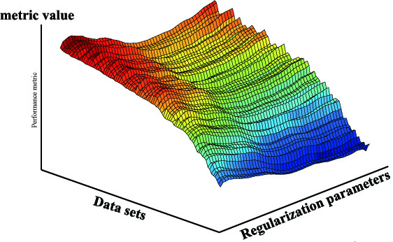
A key assumption of the proposed method is that given a regularized reconstruction formulation and a specific performance metric $$$g$$$, the nonlinear function $$$g(\lambda)$$$ is usually smooth and has a simple shape, and that the collection of all $$$g(\lambda)$$$ for different datasets should have a simple topology in a certain feature space (e.g., a smooth hypersurface illustrated in Fig. 1). Therefore, it is possible to learn this nonlinear function from prior training data.
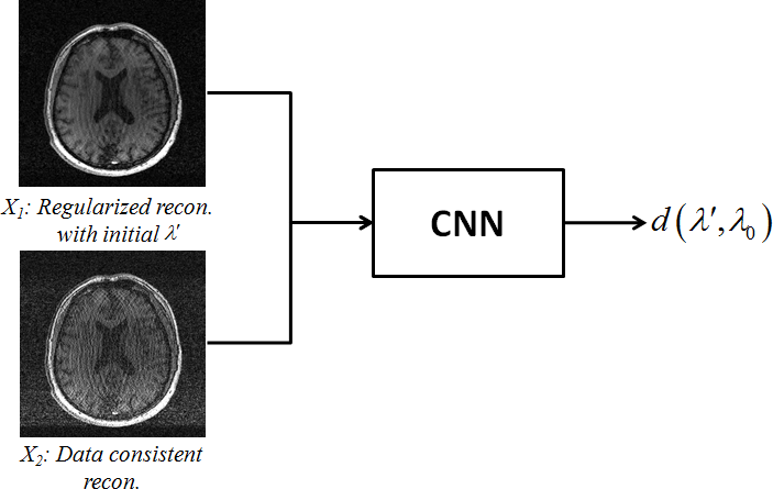
To achieve this, we propose a deep learning based method to capture such nonlinear relationship and predict the “oracle” $$$\lambda_0$$$ (corresponding to a reconstruction with optimal performance metric value) based on an initial guess of $$$\lambda$$$ (e.g., $$$\lambda’$$$). Specifically, we designed a convolutional neural network (CNN) to take two "input" images, $$$X_1$$$ and $$$X_2$$$, and output a distance measure between $$$\lambda_0$$$ and $$$\lambda’$$$ (illustrated in Fig. 2). $$$X_1$$$ is an initial reconstruction using $$$\lambda’$$$ (serving as a "reference" point) and $$$X_2$$$ is reconstructed with $$$\lambda=0$$$, representing a data consistent reconstruction. CNN is selected because it is a powerful feature extraction tool, particularly for the purpose of capturing the key features evaluated by a metric. These features are then used for determining the distance between $$$\lambda’$$$ and $$$\lambda_0$$$, such that the latter one can be predicted for new data.
It is important to note that instead of directly outputting $$$\lambda_0$$$, which can be significantly different for different datasets, we design the CNN to output a distance measure $$$d(\lambda, \lambda_0)$$$ which is insensitive to scale differences, simplifying the learning problem. Specifically, we chose $$$d(\lambda, \lambda_0)=log(\lambda/\lambda_0)$$$. To illustrate this, consider an example where $$$\lambda$$$ has a large dynamic range (e.g., [$$$10^{-1}$$$,$$$10^{-5}$$$]), and $$$\lambda’$$$ is two orders of magnitude different than $$$\lambda$$$, the log-ratio measure can shrink the difference to a reasonable numerical range (e.g., [-2, 2] with $$$\lambda_0=10^{-3}$$$). We believe this will make the learning method more stable and be equally sensitive to any initial $$$\lambda’$$$.
Materials and Methods
T1-weighted images from five different subjects were acquired on a 3T MR scanner (SIEMENS Prisma) using a 3D-FLASH sequence with the same parameters (matrix size=256$$$\times$$$256, spatial resolution=0.9mm$$$\times$$$0.9mm, slice thickness= 2mm, FA=90°, TR=20ms, TE=4.45ms). Reconstructions of each slice with different $$$\lambda'$$$ were used as different training samples.
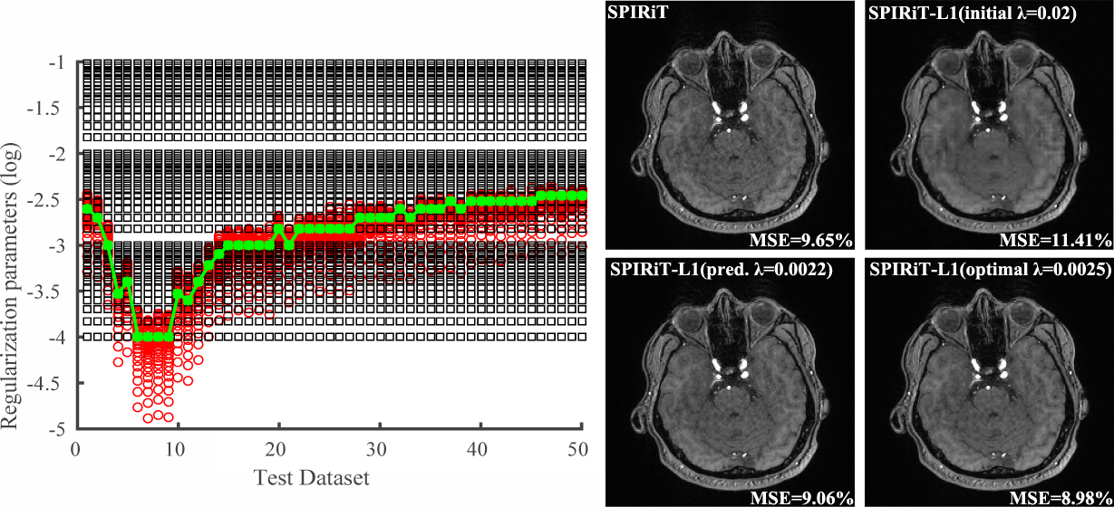
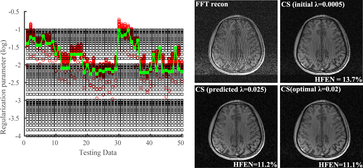
Two CNNs were trained for two different L1-regularized reconstruction methods, i.e., basic compressed sensing11 (CS) and L1-SPIRiT12, respectively. For the CS reconstruction, the optimal $$$\lambda$$$’s were selected based on high-frequency error norm (HFEN) and the data were retrospectively undersampled by $$$\times$$$2 using a 1D variable-density pattern, while for the L1-SPIRiT the optimal $$$\lambda$$$’s were selected using mean squared error (MSE) and a $$$\times$$$4 variable-density Poisson disk undersampling pattern, to demonstrate the network’s capability to learn the nonlinear relationships for different metrics.
Results and Discussion
Figure 3 shows the learned regularization parameters for L1-SPIRiT and corresponding reconstructions produced by different choices of $$$\lambda$$$. As can be seen, the learned parameters match very well with the "oracle" ones for different datasets, indicating the network’s capability in capturing the nonlinear mapping between $$$\lambda'$$$ and $$$\lambda_0$$$. The reconstruction with predicted $$$\lambda$$$ is similar to the one used $$$\lambda_0$$$ and significantly better than initial $$$\lambda'$$$. Figure 4 shows a similar comparison as in Fig. 3 for CS reconstruction, demonstrating the flexibility of the proposed method, i.e., for different reconstruction formulations and metrics.Conclusion
This work proposes a novel deep learning method for regularization parameter selection. The new method is flexible, efficient and effective; it can also be extended to other problems involving the determination of multiple parameters for any image quality metric.Acknowledgements
This work was partially supported by NIH-R21-EB021013-01, NIH-P41-EB002034 and NSFC-61671441.References
- Craven P, Wahba G. Smoothing noisy data with spline functions. Numer Math 1979;31:377–403.
- Carew JD, Wahba G, Xie X, Nordheim EV, Meyerandb ME. Optimal spline smoothing of fMRI time series by generalized crossvalidation. Neuroimage 2003;18:950–961.
- Sourbron S, Luypaert R, Schuerbeek PV, Dujardin M, Stadnik T. Choice of the regularization parameter for perfusion quantification with MRI. Phys Med Biol 2004;49:3307–3324.
- Stein C. Estimation of the mean of a multivariate normal distribution. Ann Statist 1981;9:1135–1151.
- Ramani S, Liu Z, Rosen J, Nielsen J-F, Fessler JA. Regularization parameter selection for nonlinear iterative image restoration and MRI reconstruction using GCV and SURE-based methods. IEEE transactions on image processing 2012;21:3659-3672.
- Weller DS, Ramani S, Nielsen J-F, Fessler JA. Monte carlo SURE-based parameter selection for parallel magnetic resonance imaging reconstruction. Magn Reson Med 2014;71:1760–1770.
- Ramani S, Weller DS, Nielsen J-F, Fessler JA. Non-cartesian MRI reconstruction with automatic regularization via monte-carlo SURE. IEEE transactions on medical imaging 2013;32:1411-1422.
- Karl WC. Regularization in image restoration and reconstruction. in Handbook of Image Video Processing, A. Bovik, Ed. New York: Elsevier,2005, pp. 183–202.
- Hansen PC, O’Leary DP. The use of the L-curve in the regularization of discrete ILL-posed problems. SIAM J Sci Comput 1993;14:1487–1503.
- Vogel CR. Non-convergence of the L-curve regularization parameter selection method. Inverse Problems 1996;12:535–547.
- Lustig M, Donoho D, Pauly JM. Sparse MRI: the application of compressed sensing for rapid MR imaging. Magn Reson Med 2007;58:1182–1195.
- Lustig M, Pauly JM. SPIRiT: iterative self-consistent parallel
imagingreconstruction from arbitrary k-space. Magn Reson Med 2010;64:457–471.
Figures