3379
Constrained Image Reconstruction Using a Kernel+Sparse Model1Department of Electrical and Computer Engineering, University of Illinois at Urbana-Champaign, Urbana, IL, United States, 2Beckman Institute for Advanced Science and Technology, University of Illinois at Urbana-Champaign, Urbana, IL, United States
Synopsis
Constrained image reconstruction incorporating prior information has been widely used to overcome the ill-posedness of reconstruction problems. In this work, we propose a novel "kernel+sparse" model for constrained image reconstruction. This model represents the desired image as a function of features "learned" from prior images plus a sparse component that captures localized novel features. The proposed method has been validated using multiple MR applications as example. It may prove useful for solving a range of image reconstruction problems in various MR applications where both prior information and localized novel features exist.
Introduction
Image reconstruction is known to be an ill-posed mathematical problem because most imaging operators are ill-conditioned and its feasible solutions are not unique due to finite sampling. To address this issue, constrained reconstruction incorporating prior information has been widely used. A popular approach to constrained reconstruction is to use regularization in which priori information is incorporated implicitly in a regularization functional. In this work, we propose a novel “kernel+sparse” model for constrained reconstruction. This model represents the desired image as a function of features “learned” from prior images plus a sparse component that captures localized novel features. The proposed representation has been validated using multiple MR applications as a testbed.
Method
Kernel+Sparse Model
We decompose the spatial variations of a desired image function into two terms, one absorbing prior information (using a kernel model) and the other capturing localized sparse features:
$$\hspace{14em}\rho(\boldsymbol{x}_n)=\sum_{i=1}^N\alpha_{i}k(i,n)+\tilde{\rho}(\boldsymbol{x}_n).\hspace{14em}(1)$$
The kernel component was motivated by the success of kernel models in machine learning. More specifically, this component models the desired image value at spatial location $$$\boldsymbol{x}_n$$$ as a function of a set of low-dimensional features $$$\boldsymbol{f}_n\in\mathbb{R}^m$$$:
$$\hspace{16.5em}\rho(\boldsymbol{x}_n)=\Omega(\boldsymbol{f}_n).\hspace{16.5em}(2)$$
The features $$$\{\boldsymbol{f}_n\}_{n=1}^N$$$ are learned/extracted from prior images, which leads to implicit incorporation of priori information. However, the function $$$\Omega(\cdot)$$$ is often highly complex in practice and cannot be accurately described as a linear operator in the original feature space1-2. Inspired by the "kernel trick" in machine learning, we linearize $$$\Omega(\cdot)$$$ in a high-dimensional transformed space spanned by $$$\{\phi(\boldsymbol{f}_n):\boldsymbol{f}_n\in\mathbb{R}^m\}$$$:
$$\hspace{16.0em}\Omega(\boldsymbol{f}_n)=\omega^T\phi(\boldsymbol{f}_n).\hspace{16.0em}(3)$$
In the sense of empirical risk minimization (ERM), the optimal $$$\omega$$$ should minimize the empirical risk:
$$\hspace{12.8em}r_{amp}(\omega)=\frac{1}{N}\sum_{n=1}^{N}l(\omega^T\phi(\boldsymbol{f}_n),\rho(\boldsymbol{x}_n)),\hspace{12.8em}(4)$$
where $$$l(\cdot)$$$ is some loss function (e.g., square-error loss). The well-known representer theorem ensures that this optimal $$$\omega$$$ takes the following form3:
$$\hspace{16.2em}\omega=\sum_{n=1}^N\alpha_i\phi(\boldsymbol{f}_i).\hspace{16.2em}(5)$$
Hence we obtain the kernel-based representation for $$$\rho(\boldsymbol{x}_n)$$$ as:
$$\hspace{11.7em}\rho(\boldsymbol{x}_n)=\sum_{i=1}^N\alpha_i\phi^T(\boldsymbol{f}_i)\phi(\boldsymbol{f}_n)=\sum_{i=1}^N\alpha_ik(i,n),\hspace{11.7em}(6)$$
where $$$k(i,n)=\phi^T(\boldsymbol{f}_i)\phi(\boldsymbol{f}_n)$$$ is a kernel function. However, Eq. (6) alone may bias the model towards prior information. To avoid this potential problem, we introduce a sparsity term into Eq. (6) to capture localized novel features as described in Eq. (1) with the requirement that $$$||M\{\tilde{\rho}(\boldsymbol{x}_n)\}||_0\leq{\epsilon}$$$ where $$$M(\cdot)$$$ is some sparsifying transform.
Image Reconstruction
Image reconstruction using the proposed model requires specification of the kernel function and features. In this work, we choose the radial Gaussian kernel function:
$$\hspace{13.9em}k(\boldsymbol{f}_i,\boldsymbol{f}_n)=\exp(-\frac{||\boldsymbol{f}_i-\boldsymbol{f}_n||_2^2}{2\sigma^2})\hspace{13.9em}(7)$$
which corresponds to an infinite-dimensional mapping function2. Choices of features are rather flexible, such as image intensities and edge information, making the proposed model even more powerful in absorbing a large range of priors.
The proposed kernel-based signal model results in maximum likelihood reconstruction by solving:
$$\hspace{5.7em}\{\alpha_i^*,\tilde{\rho}^*\}=\arg\max_{\{\alpha,\tilde{\rho}\}}L(d,I(\{\sum_{i=1}^{N}\alpha_ik(i,n)+\tilde{\rho}(\boldsymbol{x}_n)\})),\mathrm{s.t.}||M\{\tilde{\rho}(\boldsymbol{x}_n)\}||_0\leq{\epsilon}.\hspace{5.7em}(8)$$
where $$$d$$$ denotes the measured data, $$$I(\cdot)$$$ the imaging operator, and $$$L(\cdot,\cdot)$$$ the likelihood function.
Results
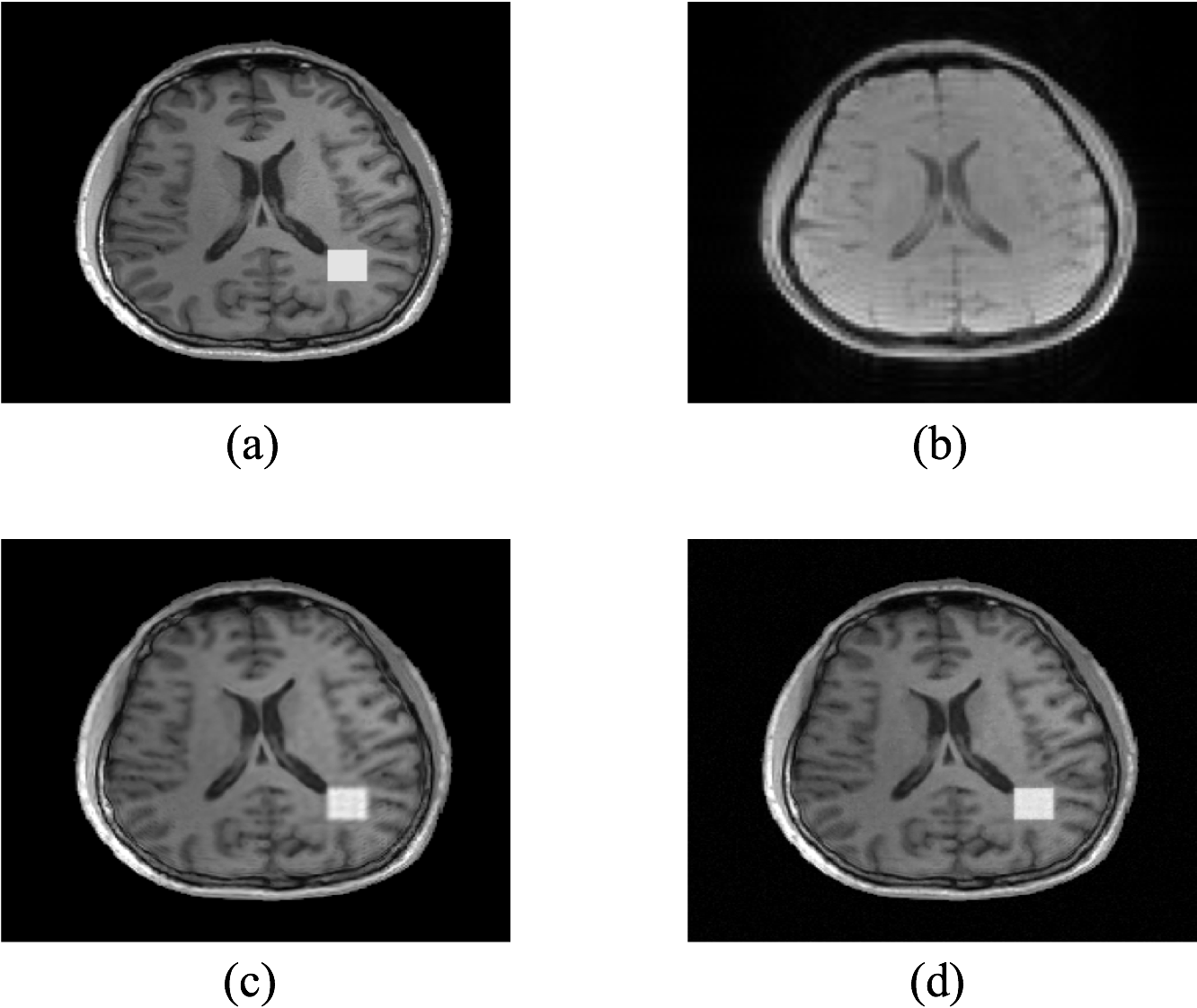
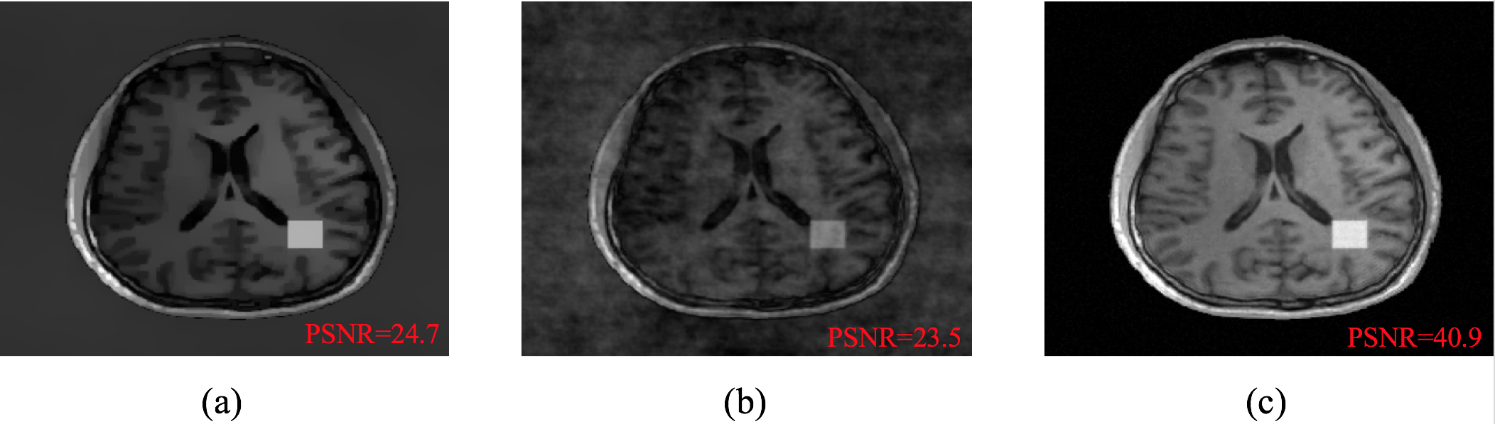
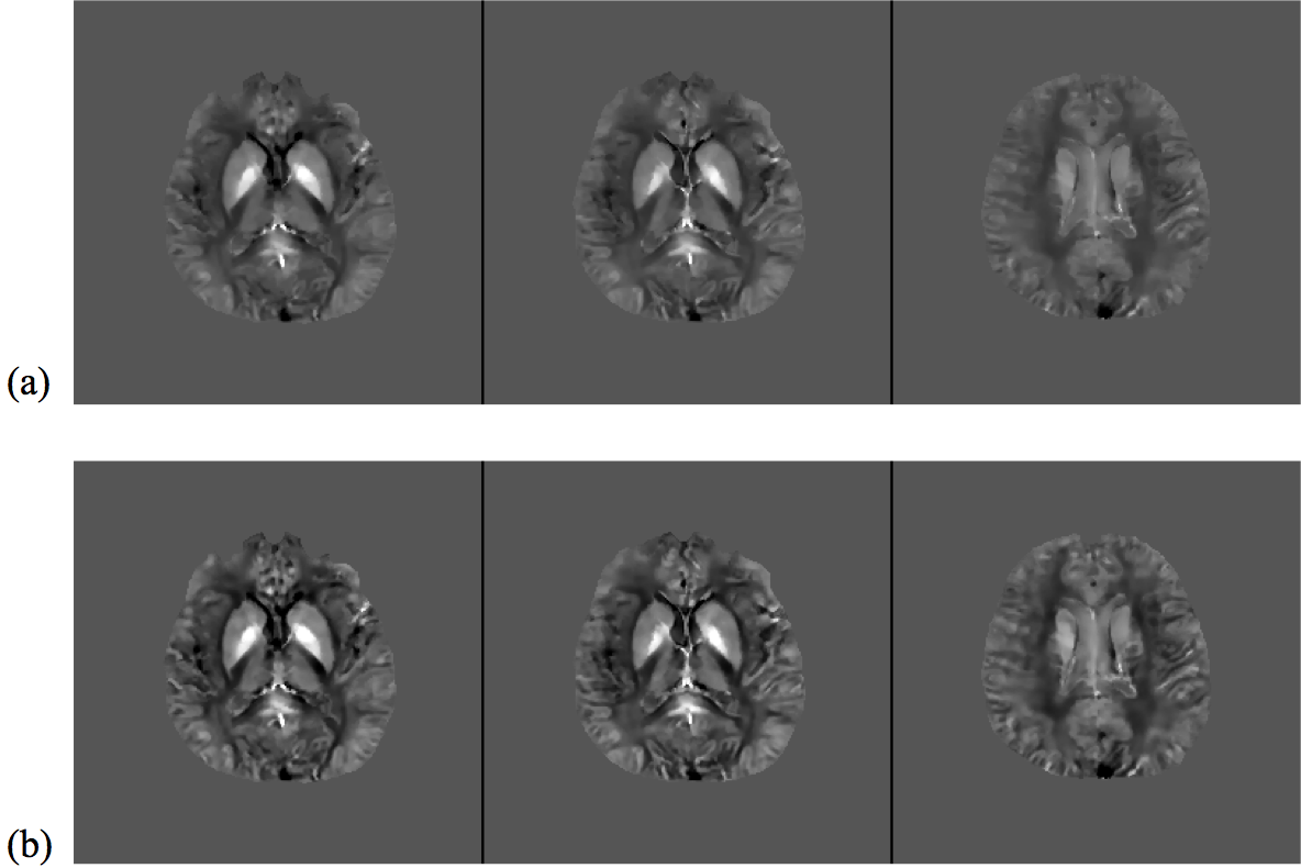
The proposed method has been evaluated in compressive sensing MRI (CS-MRI), dynamic imaging and quantitative susceptibility mapping (QSM) respectively. For CS-MRI, simulation data were generated from a T1-weighted image using variable density random sampling. A constant square was added into the image as a novel feature. Figure 1 illustrates how the sparse term in Eq. (1) protects the novel features. Figure 2 shows that the proposed method produced significantly improved reconstruction as compared to the traditional compressive sensing reconstruction and the spatially regularized reconstruction. For dynamic imaging, in vivo data were acquired from a dynamic contrast-enhanced MRI scan of breast with 20 frames and 256×256 Fourier samples, during the dynamic passage of gadolinium. Figure 3 shows that the proposed method produced less noisy reconstruction, compared to the Fourier method. For QSM, tissue-susceptibility-induced field shift is obtained by the method proposed in Ref [4] from an in vivo data acquired using the SPICE technique5, with 230×230×72 mm3 FOV and 96×110×24 matrix size. Figure 4 shows the proposed method significantly improved the estimated susceptibility map with clearer tissue contrast and better-defined edges than the conventional method6.Conclusions
This paper introduces a novel “kernel+sparse” model for constrained image reconstruction. This model effectively absorbs prior information into the kernel term while protects its ability to capture localized novel features. The proposed method has been evaluated in multiple applications, producing impressive results. It may prove useful for solving a range of constrained image reconstruction problems in various MRI applications where both prior information and localized novel features exist.Acknowledgements
This work was supported in part by the following grants: NIH-R21-EB021013-01 and NIH-P41-EB002034.References
1. Hofmann, T., Schölkopf, B., & Smola, A. J. (2008). Kernel methods in machine learning. The annals of statistics, 1171-1220.
2. Wang, G., & Qi, J. (2015). PET image reconstruction using kernel method. IEEE transactions on medical imaging, 34(1), 61-71.
3. Schölkopf, B., Herbrich, R., & Smola, A. (2001). A generalized representer theorem. In Computational learning theory (pp. 416-426). Springer Berlin/Heidelberg.
4. Peng, X., Lam, F., Li, Y., Clifford, B., & Liang, Z. P. (2017). Simultaneous QSM and metabolic imaging of the brain using SPICE. Magnetic Resonance in Medicine.
5. Lam, F., Ma, C., Clifford, B., Johnson, C. L., & Liang, Z. P. (2016). High‐resolution 1H‐MRSI of the brain using SPICE: Data acquisition and image reconstruction. Magnetic resonance in medicine, 76(4), 1059-1070.
6. Liu,
T., Liu, J., De Rochefort, L., Spincemaille, P., Khalidov, I., Ledoux, J. R.,
& Wang, Y. (2011). Morphology enabled dipole inversion (MEDI) from a single‐angle acquisition: comparison with COSMOS in
human brain imaging. Magnetic resonance in medicine, 66(3), 777-783.
Figures