Synopsis

MR Fingerprinting offers the ability to obtain simultaneous tissue (T1,T2…) and hardware (B1, B0…) parameter maps in a fast acquisition time but is limited by the size of the reconstruction dictionary. In previous work we demonstrated that these issues can be overcome by reconstructing the data using a properly trained neural network. Here we characterize the accuracy of a neural network trained on sparse dictionaries for reconstruction of noisy data.

Introduction

Accurate reconstruction of MR Fingerprinting (MRF) (1) data requires matching the data to a large dictionary comprised of the signal magnetization from all possible tissue parameters combinations. Dictionary size grows exponentially and can quickly become impractically large in multi-parametric applications (2,3). Instead of matching to a dictionary, we’ve previously demonstrated (4) the feasibility of fast and accurate reconstruction of MRF data by a neural network (NN) trained with Deep Learning algorithms. Deep Learning (DL) reconstruction can eliminate the need for large reconstruction dictionaries. In this work we characterize the accuracy of a DL reconstruction of noisy MRF data using heavily undersampled training dictionaries.

Methods

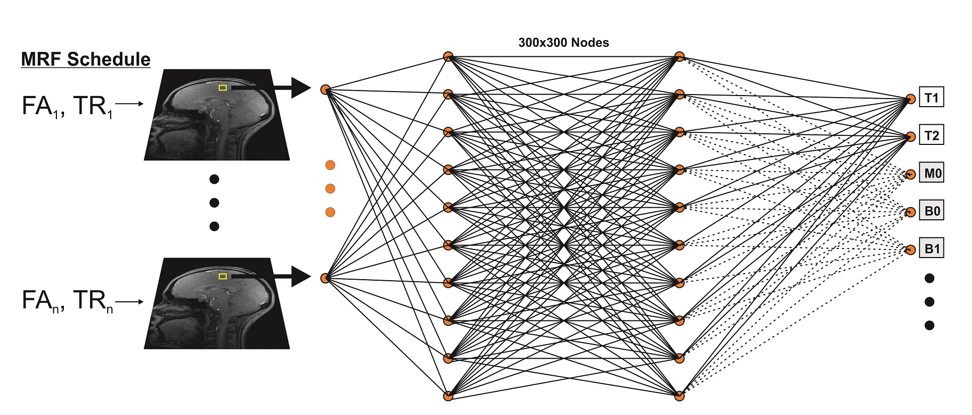
A four layer fully-connected neural network composed of input and output layers and two hidden layers was defined using the TensorFlow framework (5) as shown in Fig. 1. The input layer consisted of 25 nodes to correspond to the 25-point trajectory of magnitude images acquired with our optimized echo-planar imaging (EPI) MRF sequence (6). Each of the two hidden layers had 300 nodes. The network was trained by the ADAM stochastic gradient descent algorithm (7). The training loss function was a defined as the mean square error. A hyperbolic tangent (tanh) function was used as the activation function of the hidden layers and a sigmoid function used for the output layer.

All experiments in this study used a modified gradient-echo EPI MRF pulse sequence whose flip angles (FA) and repetition times (TR) were set according to an optimized measurement schedule, as previously described (6,8,9).

The network was trained with an initial dictionary of ~79,900 entries consisting of T1 in the range 1-5000 ms and T2 values in the range (1-2000) ms, excluding entries where T1 < T2. The magnetization due to each (T1, T2) pair was calculated by Bloch equation simulation using the Extended Phase Graph formalism (10,11). Gaussian noise with 2% standard deviation and zero mean was added to the training dictionary. This dictionary was used to train the network for 1000 epochs on an Nvidia K80 GPU with 2 GB of memory.

The effect of the training dictionary density on the resulting reconstruction error was measured by sub-sampling the initial dictionary variously from 2 to 60 fold. The network was then trained with each sub-sampled dictionary and used to reconstruct the initial, fully sampled dictionary whose entries were corrupted by zero mean Gaussian noise with 0 (no noise) or 0.5% standard deviation. This was repeated 10 times for each undersampling factor to allow statistical calculations. The NN reconstruction was also compared to a conventional MRF dictionary matching reconstruction by matching the initial, fully sampled dictionary to each sub-sampled dictionary and calculating the resultant error. The mean and standard deviation of the RMSE of the reconstructed T1 and T2 maps of each reconstruction method was then calculated as a function of the dictionary sub-sampling factor.

Results

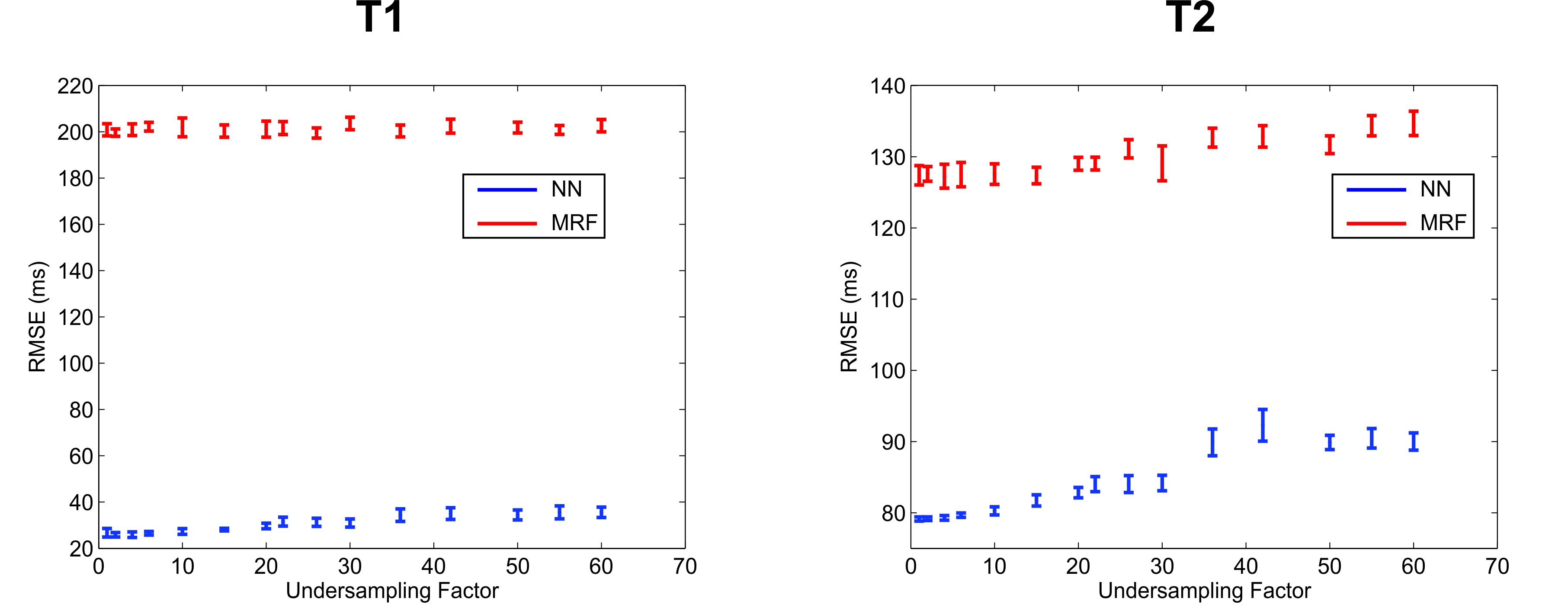
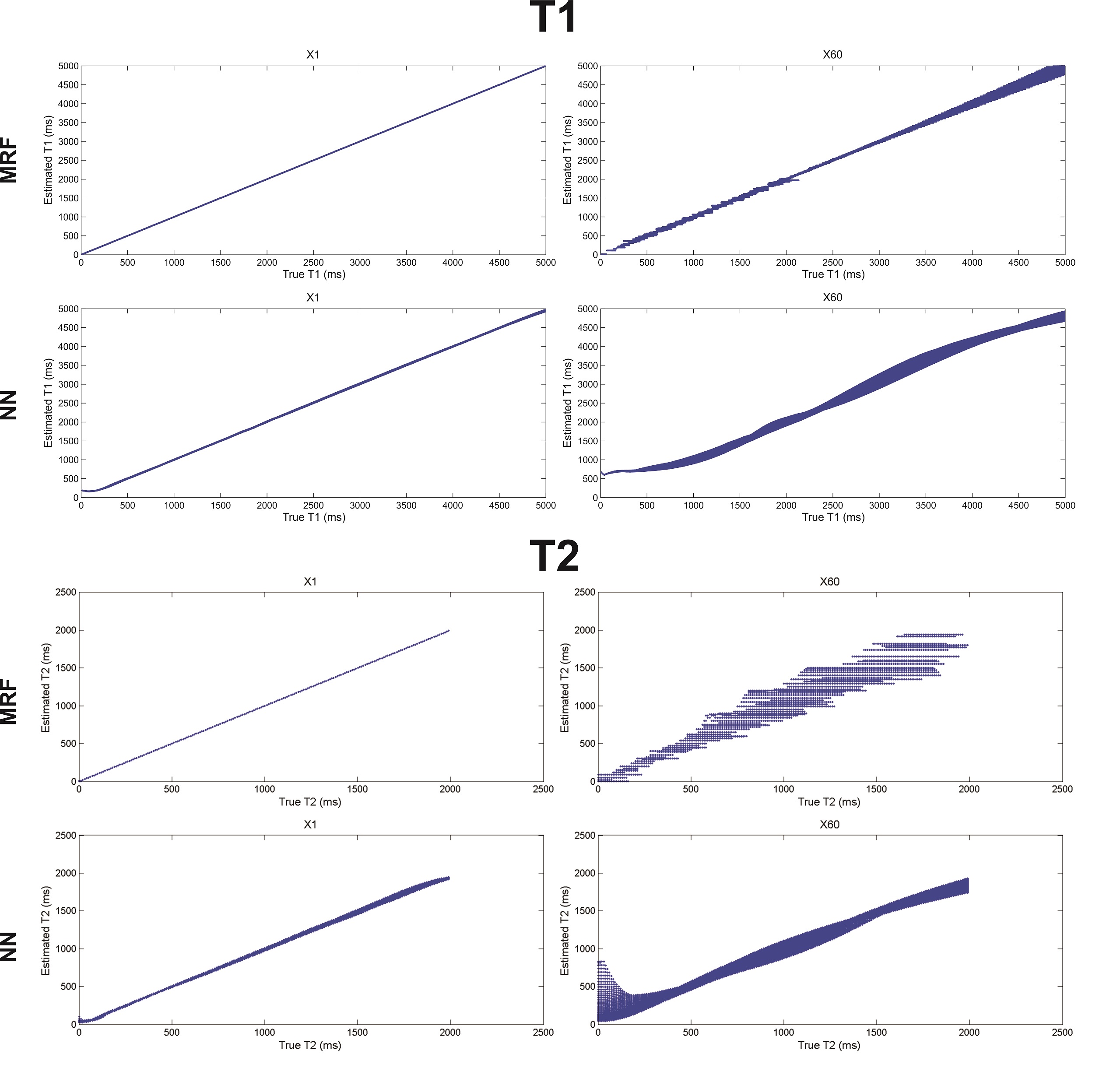
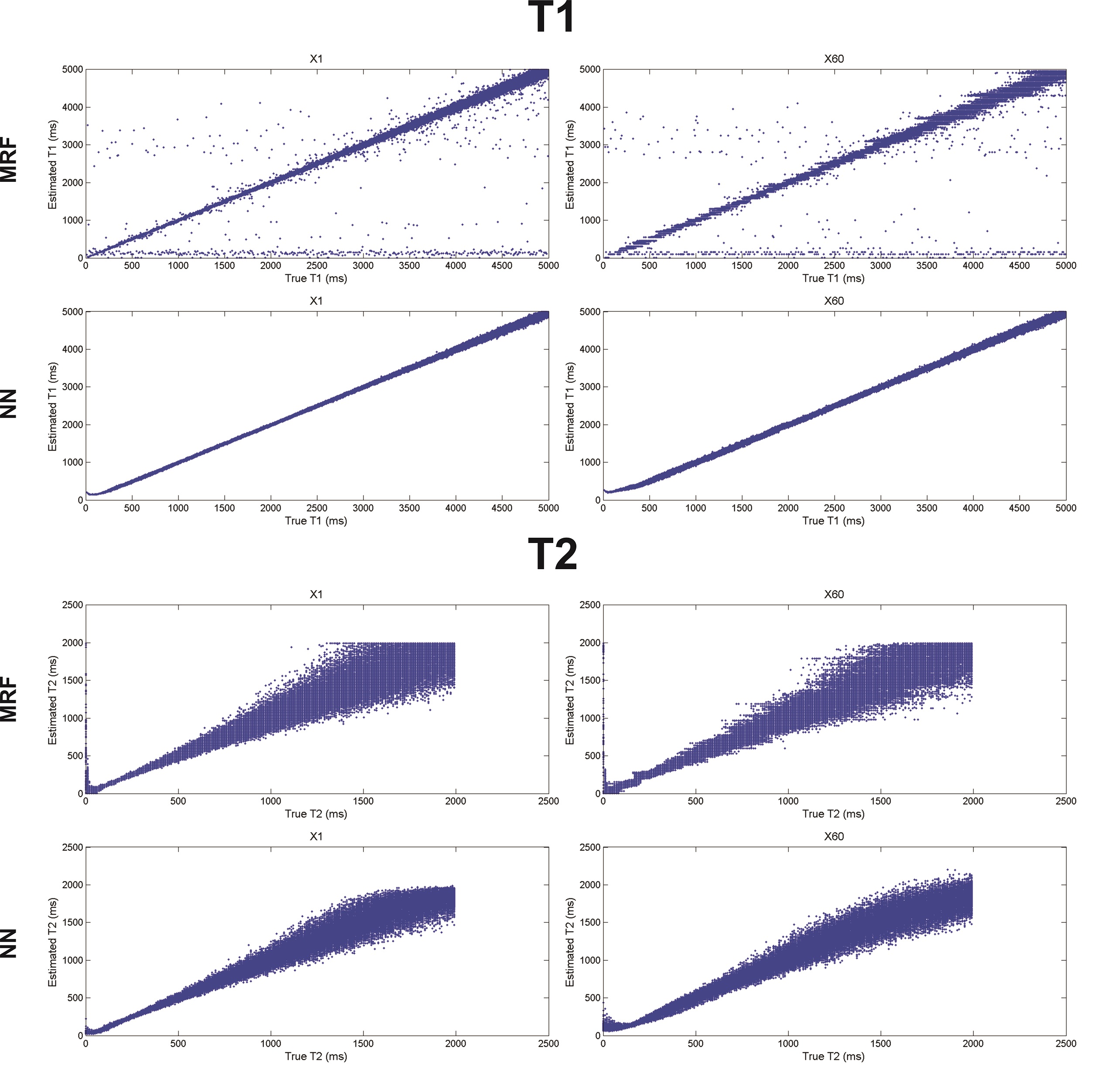
The mean T1 and T2 RMSEs across the ten repetitions are shown as a function of the dictionary undersampling factor in Fig. 2. The RMSE of the NN reconstruction grew with increasing undersampling, as expected, but was approximately 5-7 fold smaller for T1 and 2 fold smaller for T2, for all undersampling factors, than the relatively constant RMSE of the conventional dictionary matching. The growth in the NN reconstruction error was well fit (R2 = 0.94 for T1 and R2=0.89 for T2) by a linear function. The reconstructed and true T1 and T2 values for the fully sampled (×1) and 60-fold undersampled (×60) dictionaries are shown in Fig. 3 for the NN and MRF reconstructions for the noise-free case and in Fig. 4 for the noisy case.

Discussion and Conclusion

The NN reconstruction is more robust to noise than conventional dictionary matching approach because the signal-to-parameter mapping is forced to be expressed in low-dimensional space and is thus insensitive to small corruptive input perturbations. The results shown in Fig. 2 indicate that the NN reconstruction error grew linearly with the dictionary sub-sampling factor. Conventional dictionary matching does not learn a functional mapping, relying instead on the similarity between the normalized measured data and the corresponding normalized dictionary entry. An unfortunate side-effect of the normalization is that noisy signals, arising from tissues with short T1 or T2 for example, are amplified and then matched to some dictionary entry leading to increased reconstruction errors (Fig. 3). In contrast, the network was trained on noisy signals and consequently yielded smaller error for both T1 and T2 than dictionary matching of the same noisy data.

Acknowledgements

References

1. Ma D, Gulani V, Seiberlich N, Liu K, Sunshine JL, Duerk JL, Griswold MA. Magnetic resonance fingerprinting. Nature 2013;495:187–192. doi: 10.1038/nature11971.

2. Su P, Mao D, Liu P, Li Y, Pinho MC, Welch BG, Lu H. Multiparametric estimation of brain hemodynamics with MR fingerprinting ASL. Magn. Reson. Med. 2016.

3. Cohen O, Huang S, McMahon MT, Rosen MS, Farrar CT. Rapid and Quantitative Chemical Exchange Saturation Transfer (CEST) Imaging with Magnetic Resonance Fingerprinting (MRF). ArXiv Prepr. ArXiv171006054 2017.

4. Cohen O, Zhu B, Matthew R. Deep Learning for Fast MR Fingerprinting Reconstruction. In: Proceedings of the International Society of Magnetic Resonance in Medicine. Honolulu, HI; 2017. p. 7077.

5. Abadi M, Agarwal A, Barham P, et al. Tensorflow: Large-scale machine learning on heterogeneous distributed systems. ArXiv Prepr. ArXiv160304467 2016.

6. Cohen O, Rosen MS. Algorithm comparison for schedule optimization in MR fingerprinting. Magn. Reson. Imaging 2017.

7. Kingma D, Ba J. Adam: A method for stochastic optimization. ArXiv Prepr. ArXiv14126980 2014.

8. Cohen O, Sarracanie M, Armstrong BD, Ackerman JL, Rosen MS. Magnetic resonance fingerprinting trajectory optimization. In: Proceedings of the International Society of Magnetic Resonance in Medicine. Milan, Italy; 2014. p. 0027.

9. Cohen O, Sarracanie M, Rosen MS, Ackerman JL. In Vivo Optimized MR Fingerprinting in the Human Brain. In: Proceedings of the International Society of Magnetic Resonance in Medicine. Singapore; 2016. p. 0430.

10. Weigel M. Extended phase graphs: Dephasing, RF pulses, and echoes-pure and simple. J. Magn. Reson. Imaging 2015;41:266–295.

11. Jiang Y, Ma D, Seiberlich N, Gulani V, Griswold MA. MR fingerprinting using fast imaging with steady state precession (FISP) with spiral readout. Magn. Reson. Med. 2015;74:1621–1631.