Introduction

The presented work aims to develop a new parallel imaging reconstruction framework based on deep neural networks for imaging acceleration. The proposed approach uses a conditional generative adversarial network (conditional GAN¹) to reconstruct images from multi-channel undersampled imaging data. This network model is trained using a loss function with an adversarial term associated with the machine learning process and a data fidelity term associated with the MRI physics. In the experiments performed in this work, the new approach does not show significant performance degradation with the increase of undersampling factors like conventional parallel imaging methods. It is likely that image reconstruction based on neural network may benefit MRI when a high undersampling factor is used.

Methods

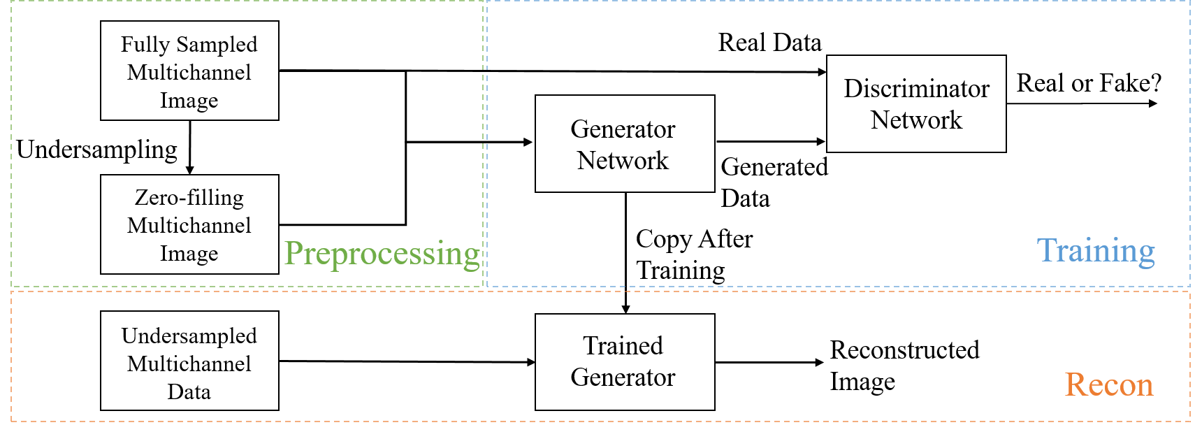
As illustrated in Figure 1, a conditional GAN is trained to reconstruct images from multi-channel undersampled data. This model consists of two sub-networks: a discriminator network $$$D$$$ which identifies if the image is real or fake with a probabilistic output between 0 (fake) and 1 (real) and a generator network $$$G$$$ which synthesizes fake images to fool the discriminator. In the presented work, these sub-networks are constructed with the same architectures as those in Radford et al². Here a mapping from the input, a set of undersampled images $$$x$$$ with noise $$$z$$$, to the output, a set of aliasing-free images $$$y$$$ is modelled as $$$G: \{x,z\} \rightarrow y$$$, where the images and the noise each follow a certain probability distribution, i.e., $$$x,y\sim p_{data}(x,y),z\sim p_z(z)$$$. The training may be formulated as a min-max problem between the generator and discriminator with an adversarial loss: $$Equation~1: \min_G\max_DL_{cGAN}(G,D)={\mathbb{E}}_{x,y\sim p_{data}(x,y)}[\log D(x,y)]+{\mathbb{E}}_{x\sim p_{data}(x),z\sim p_z(z)}[\log(1-D(x,G(x,z)))] $$This loss function represents an adversarial judgement made by the discriminator: The discriminator tends to accept the real image ($$$y$$$). However, when the generator is attempting to output an image as close to the real image as possible during the training, the discriminator would endeavor to reject this output because it is generated from a fake image ($$$x$$$). By optimizing the min-max loss, the two sub-networks will reach an agreement: The discriminator will produce a probabilistic degree of the reality while the generator will minimize the gap between generated images and real images. In addition to this machine learning process, it is important that a physical data-fidelity constraint should be applied, i.e., the generator should output images close to the corresponding ground truth images in an L1 sense: $$Equation~2: \min_GL_1(G)={\mathbb{E}}_{x,y\sim p_{data}(x,y),z\sim p_z(z)}||y-G(x,z)||_1$$The final objective loss combines the loss terms in Equation 1 (related to machine learning) and 2 (related to MRI physics): $$Equation~3: \min_G\max_DL_{cGAN}(G,D)+\alpha L_1(G)$$where $$$\alpha$$$ is a weighting factor for balancing two losses. Standard backpropagation and stochastic gradient descent algorithms are used to minimize the objective loss during the training process. To validate the proposed approach, a series of 3D brain images (FOV 240$$$\times$$$240$$$\times$$$220mm, axial resolution 256$$$\times$$$256 with 10~70 slices) was collected with an 8-channel coil array from 10 healthy volunteers. These images were converted to a total of 290 sets of multi-channel 2D data for image reconstruction experiments. Among these data, 70%, 10% and 20% were used respectively for training, validation and test. The data were uniformly undersampled to simulate imaging acceleration. SENSE³ and GRAPPA⁴ were used as reference approaches.

Results

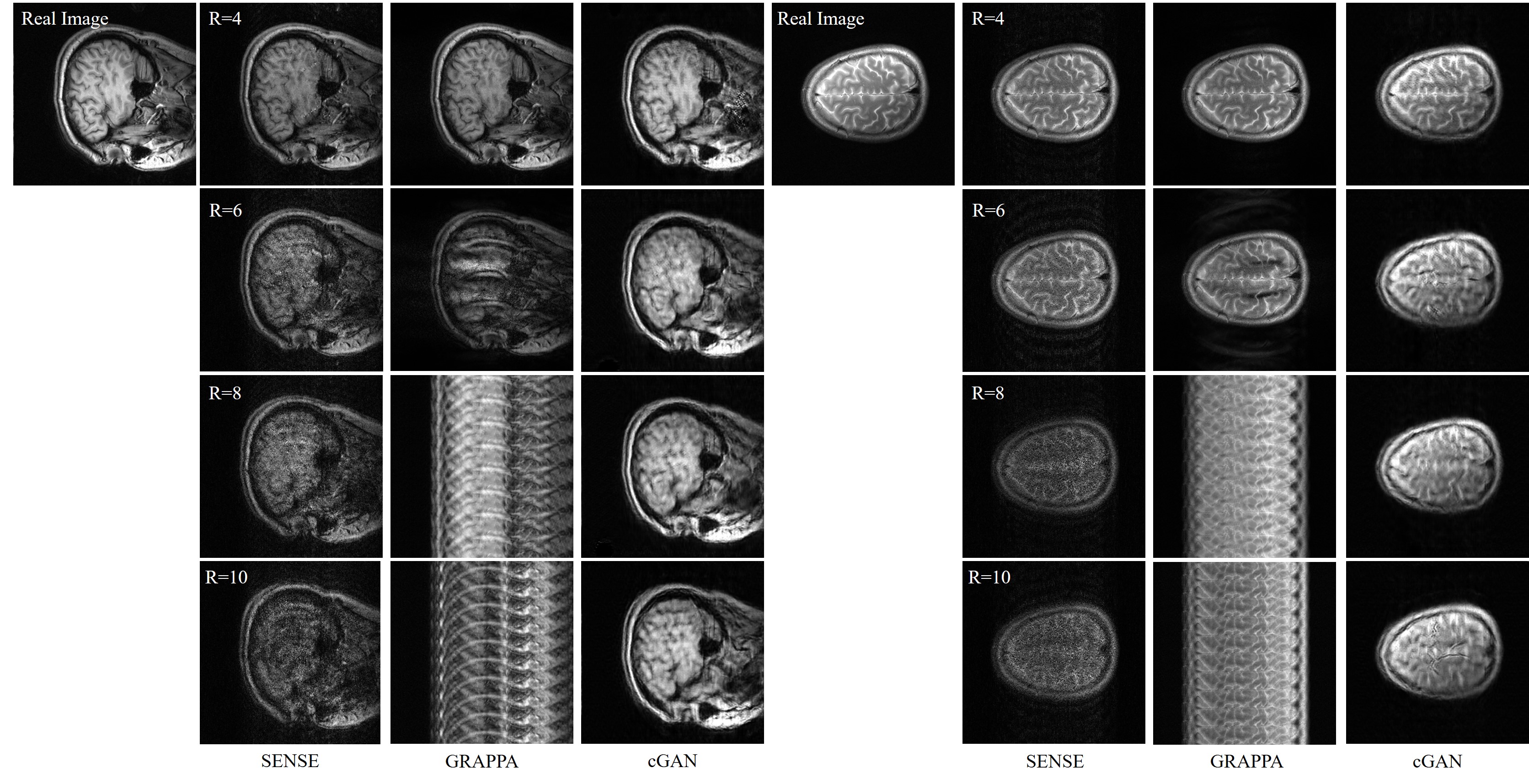
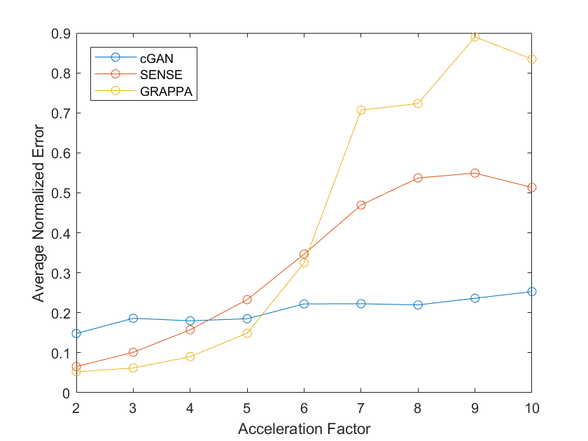
Figure 2 gives two examples of reconstructed images with different imaging acceleration factors. When a low acceleration factor (≤4) is used, the conditional GAN gives reconstruction slightly worse than SENSE and GRAPPA. When a high acceleration factor (>4) is used, the conditional GAN performs better than SENSE and GRAPPA. A quantitative comparison is given in Figure 3, which shows the plots of reconstruction errors against acceleration factors. It can be seen that the conditional GAN gives errors that slightly increase with acceleration factors. In comparison, SENSE and GRAPPA gives errors that increase dramatically with acceleration factors.

Discussion

Parallel imaging relies on a mathematical model where g-factor plays an important role. As g-factor increases fast with less data, the performance of SENSE and GRAPPA is sensitive to the increase of acceleration factors. It is likely that neural networks can learn image structures from a large amount of data. Aliasing is treated as outliers and may be removed from images.This image reconstruction mechanism is more dependent on how well the neuronal networks are trained. As a result, the conditional GAN gives performance less sensitive to acceleration factors. When a high acceleration factor is used, parallel imaging typically suffers from the increase of g-factor and neural network method may offer some advantages.

Conclusion

A new image reconstruction approach based on deep learningis developed to accelerate MRI. It is likely that this approach is suitable for image reconstruction from highly undersampled data when parallel imaging suffers from a high g-factor.

Acknowledgements

This work is supported by NIH R01EB022405.