3367
Image Reconstruction of Accelerated Dynamic MRI using Spatiotemporal Dictionaries with Global Sparsity Regularization1Institute for Biomedical Engineering, ETH Zurich, Zurich, Switzerland
Synopsis
Adaptive spatiotemporal dictionaries offer improved reconstruction accuracy for dynamic cardiac MRI. However, most modern methods perform local encoding of image patches treating them independently. In order to increase reconstruction quality, we present a convex model that allows global control of encoding sparsity. The proposed method has a single tunable parameter and delivers 9% peak signal-to-noise ratio improvement of reconstruction compared to the state-of-the-art dictionary-based approach. Moreover, the implemented numerical scheme allowed 3-fold reconstruction time reduction.
Introduction
Compressed sensing theory enables efficient reconstruction of undersampled magnetic resonance (MR) data [1], yielding reduced acquisition time. Dictionary learning methods allow to learn data adaptive transforms where the considered type of signals have a sparse representation, hence resulting in a more accurate reconstruction [2]. Given a learned dictionary, sparse reconstruction is a nontrivial problem. Modern algorithms use orthogonal matching pursuit for locally sparse signal encoding. In this work, we propose a convex relaxation of MR image reconstruction that performs joint sparse encoding of spatiotemporal image patches balancing sparsity level globally. We compare our method to the state-of-the-art reconstruction method: Dictionary Learning with Temporal Gradients (DLTG) [3] using cardiac cine MRI data.Methods
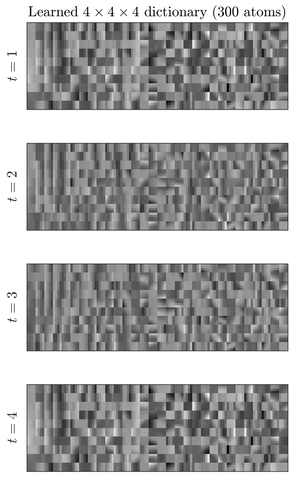
Dynamic 2D cardiac MRI datasets were acquired on 1.5 and 3T systems (Philips Healthcare, Best, The Netherlands) with voxel size of 1.4x1.4x8 mm3 and 25 dynamics, yielding 375 short-axis scans of size $$$N_d=128\times128\times25$$$ pixels. Following Caballero et al. [3], we use spatiotemporal patches of $$$4\times4\times4=N_p$$$ size and set the size of the dictionary to $$$N_a=300$$$. Since the dictionary is learned on fully sampled data, we used an efficient implementation of the generic online dictionary learning algorithm [4] provided by the Sklearn package [5], which iteratively solves the following optimization problem:
$$\min_{D\in\mathbb{R}^{N_p\times N_a}, U\in\mathbb{R}^{N_a\times N_s}} \frac12 \|DU − Y\|_{2,2}^2 + \alpha\|U\|_{1,1},\qquad\text{s.t.}\quad\|D_k\|_2=1,\quad k=1,\dots,N_a.\qquad(1)$$
Where $$$Y$$$ are training patches extracted from fully sampled data, $$$U$$$ is the matrix of patch encodings, $$$D$$$ is the learned dictionary, and the regularization parameter $$$\alpha=0.4$$$. We use the overcomplete discrete cosine transform as an initialization for $$$D$$$ and conduct 1000 iterations with 2000 patches in each batch. The resulting dictionary is shown in Figure 1. During reconstruction, the sparsity measure was relaxed to convex L1 norm, yielding the following constrained optimization problem:
$$\min_{U, X} \|U\|_{1,1} + \mathcal{I}[\|\mathcal{P}(X) - DU\|_{2,2} \leq \varepsilon],\quad\text{s.t.} \quad M_iFX_i=b_i, \quad i=1,\dots,N_t.\qquad(2)$$
Here indicator $$$\mathcal{I}[condition]=0$$$ when $$$condition$$$ is fulfilled and is $$$+\infty$$$ otherwise, $$$M_i$$$ and $$$b_i$$$ are undersampling matrices and k-spaces, respectively. The orthogonal linear operator $$$\mathcal{P}$$$ implements patch extraction (with circulant wrapping) from the given 2D+t image, while its adjoint $$$\mathcal{P}^T$$$ reconstructs an image from a patch representation by averaging of overlaps. Parameter $$$\varepsilon$$$ limits the global residual between the original signal and its sparse representation. Low values of $$$\varepsilon$$$ yield a sparser solution, while high values of $$$\varepsilon=10^{−5}N_d$$$ allow to account for noise in the k-space measurements $$$b_i$$$. To solve the problem (2) we cast it to the equivalent optimization problem
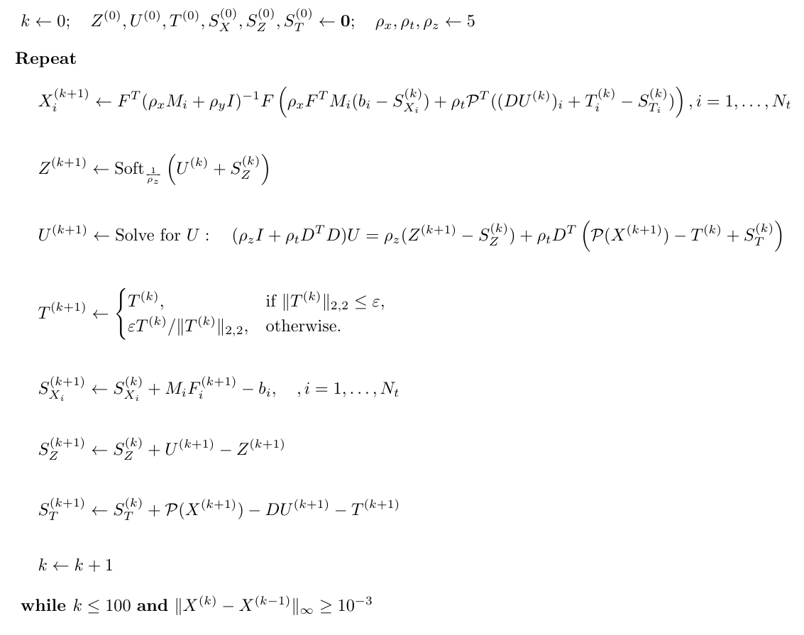
$$\min_{U,X,Z,T} \|Z\|_{1,1} + \mathcal{I}[\|T\|_{2,2} \leq \varepsilon],\quad\text{s.t.} \; M_iFX_i=b_i,\,i=1,\dots,N_t,\quad U = Z,\quad\mathcal{P}(X)-DU=T.\qquad(3)$$
Problem (3) can be solved efficiently with the ADMM algorithm [6] as described in Figure 2. We will further refer to the proposed reconstruction method as GSDR (Globally Sparse Dictionary based Reconstruction).
Results
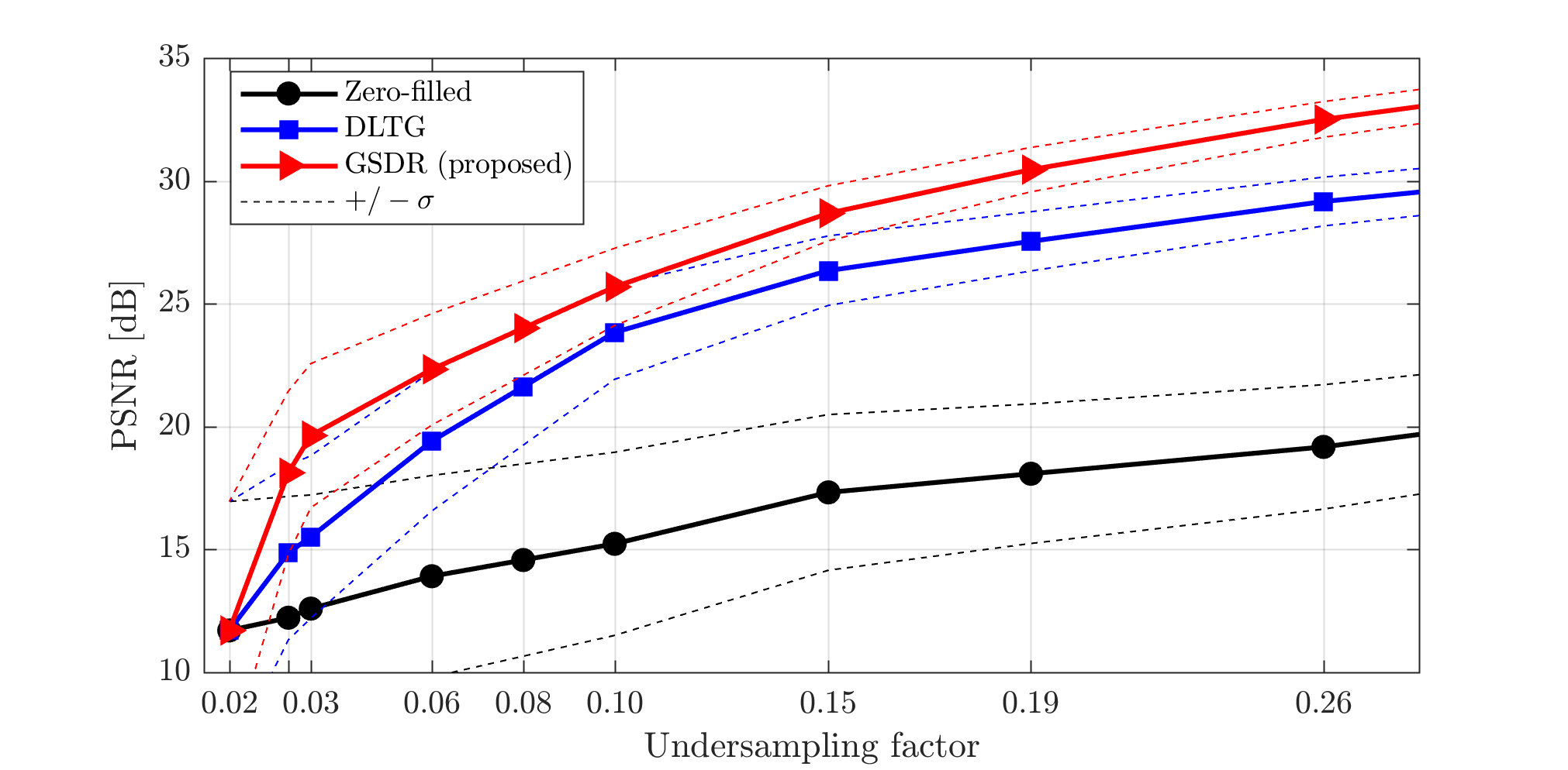
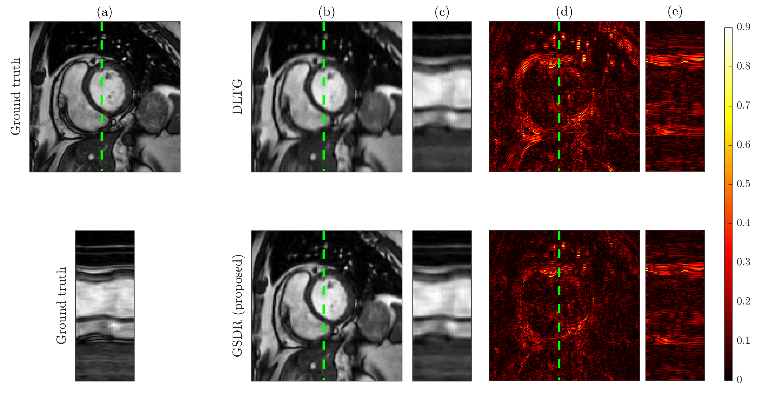
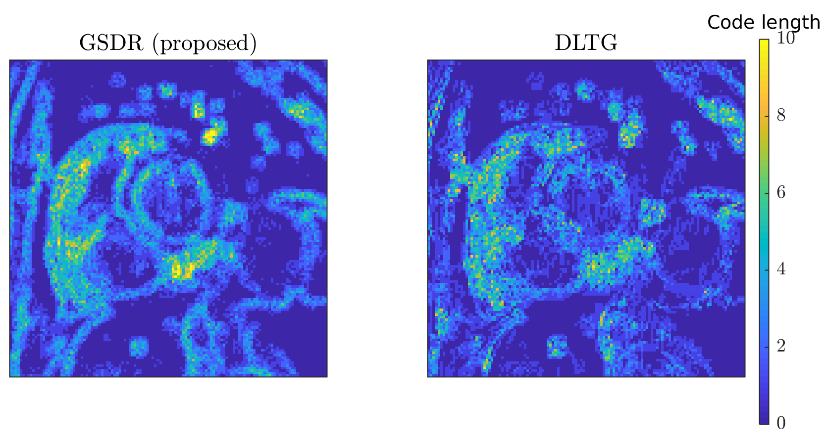
We compared the proposed algorithm to the state-of-the-art dictionary-based reconstruction with local sparsity constraints DLTG [3] for retrospectively undersampled data. The same dictionary was used for both methods. Figure 3 shows that the proposed method provides more accurate reconstruction in terms of (peak SNR) PSNR for all acceleration factors. Visual inspection of reconstructed images (Figure 4) indicates higher image sharpness of GSDR results. Encoding allocation patterns illustrated in Figure 5 reveal the consequences of the proposed global sparsity: the method tends to allocate more atoms to describe regions that contain large motion or sharp edges, and limits the code length for static or homogeneous regions. The run times of the proposed GSDR and DLTG methods were 9 and 28 minutes respectively on a 3.8 GHz Intel Core i7 CPU.Conclusion
In this work, we have developed an efficient reconstruction method based on adaptive spatiotemporal dictionaries and global sparsity constraints. The method has a single tunable parameter that allows controlling sparsity level and noise tolerance. The proposed approach achieved 9% PSNR improvement compared to the state-of-the-art DLTG reconstruction for dynamic cardiac MRI with an undersampling factor of up to 6.7. Moreover, the implemented numerical scheme allowed 3-fold reconstruction time reduction.Acknowledgements
The authors acknowledge funding from the European Union’s Horizon 2020 research and innovation programme under grant agreement No 668039.References
[1] Lustig M, Donoho D, Pauly JM. Sparse MRI: The application of compressed sensing for rapid MR imaging. Magnetic resonance in medicine. 2007;58(6):1182-95.
[2] Schmidt J, Kozerke S. Dynamic cardiac MR image reconstruction models using machine learning on large training data sets. ISMRM 2017.
[3] Caballero J, Price AN, Rueckert D, Hajnal JV. Dictionary learning and time sparsity for dynamic MR data reconstruction. IEEE transactions on medical imaging. 2014;33(4):979-94.
[4] Mairal J, Bach F, Ponce J, Sapiro G. Online dictionary learning for sparse coding. InProceedings of the 26th annual international conference on machine learning 2009. (pp. 689-696). ACM.
[5] Pedregosa F, Varoquaux G, Gramfort A, Michel V, Thirion B, Grisel O, Blondel M, Prettenhofer P, Weiss R, Dubourg V, Vanderplas J. Scikit-learn: Machine learning in Python. Journal of Machine Learning Research. 2011;12:2825-30.
[6] Boyd S, Parikh N, Chu E, Peleato B, Eckstein J. Distributed optimization and statistical learning via the alternating direction method of multipliers. Foundations and Trends® in Machine Learning. 2011;3(1):1-22.
[7] Parikh N, Boyd S. Proximal algorithms. Foundations and Trends® in Optimization. 2014 Jan 13;1(3):127-239.
Figures