3364
Reconstruction of synthetic T1 MPRAGE via Deep Neural Network from Multi Echo Gradient Echo images.1Yonsei University, Seoul, Republic of Korea, 2Seoul St. Mary's Hospital, College of Medicine, The Catholic University of Korea, Seoul, Republic of Korea
Synopsis
We propose to use deep learning to reconstruct synthetic T1-weighted Magnetization prepared rapid gradient echo (MPRAGE) image from multi echo gradient echo (mGRE) images. With our method, high tissue contrast can be achieved without actual MPRAGE scan, which could be utilized for post processing methods, such as tissue segmentation or volumetric quantification. We validated our method’s accuracy by comparing the result of synthetic images with the true image via segmentation and volumetry. Additionally, we tested our method on clinical images containing pathologies not seen in the training set.
Introduction
Three-dimensional (3D) multi-echo gradient echo (mGRE) imaging has been widely used due to its fast scan time and rich susceptibility contrasts. Recently, 3D mGRE imaging has been utilized to produce susceptibility weighted images or quantitative susceptibility mapping for both clinical and research purposes [1,2]. However, mGRE protocol optimized for these susceptibility related contrasts imaging has insufficient tissue contrast between brain tissues. To supplement this, in many research protocols, T1-weighted Magnetization prepared rapid gradient echo (MPRAGE) images are additionally acquired for automatic region of interest analysis. Moreover, the acquired MPRAGE images also can be utilized for volumetric quantification, cortical thickness measurement or image registration.However, as this requires additional scan time, several attempts have been made to generate highly T1-weighted from mGRE data itself [3,4]. Here, we propose to use deep learning method to reconstruct synthetic T1-weighted MPRAGE image from mGRE images. To evaluate the utility of our method, we compared the volumetry result of synthetic images with the actual images. In addition, we tested our method on clinical images containing pathologies not seen in the training set.Method
Data acquisition
22 healthy volunteers were scanned at 3T MRI. MR images of two patients were retrospectively collected for additional validation. Parameters for mGRE were voxel size = 0.8 x 0.8 x 2 mm3, TR = 30 ms, TE = 7.20, 13.6, 20.0, 26.4 ms for 4 echoes, flip angle = 17°. For MPRAGE, voxel size = 1 x 1 x 1 mm3, TR = 6.8 ms TE = 1.5 ms, TI = 1100 ms, FA = 7°, parallel imaging factor of 2 were used for both sequences. Total scan time was 3 min 16 s for mGRE and 5 min 21 s for MPRAGE.
Deep neural network training
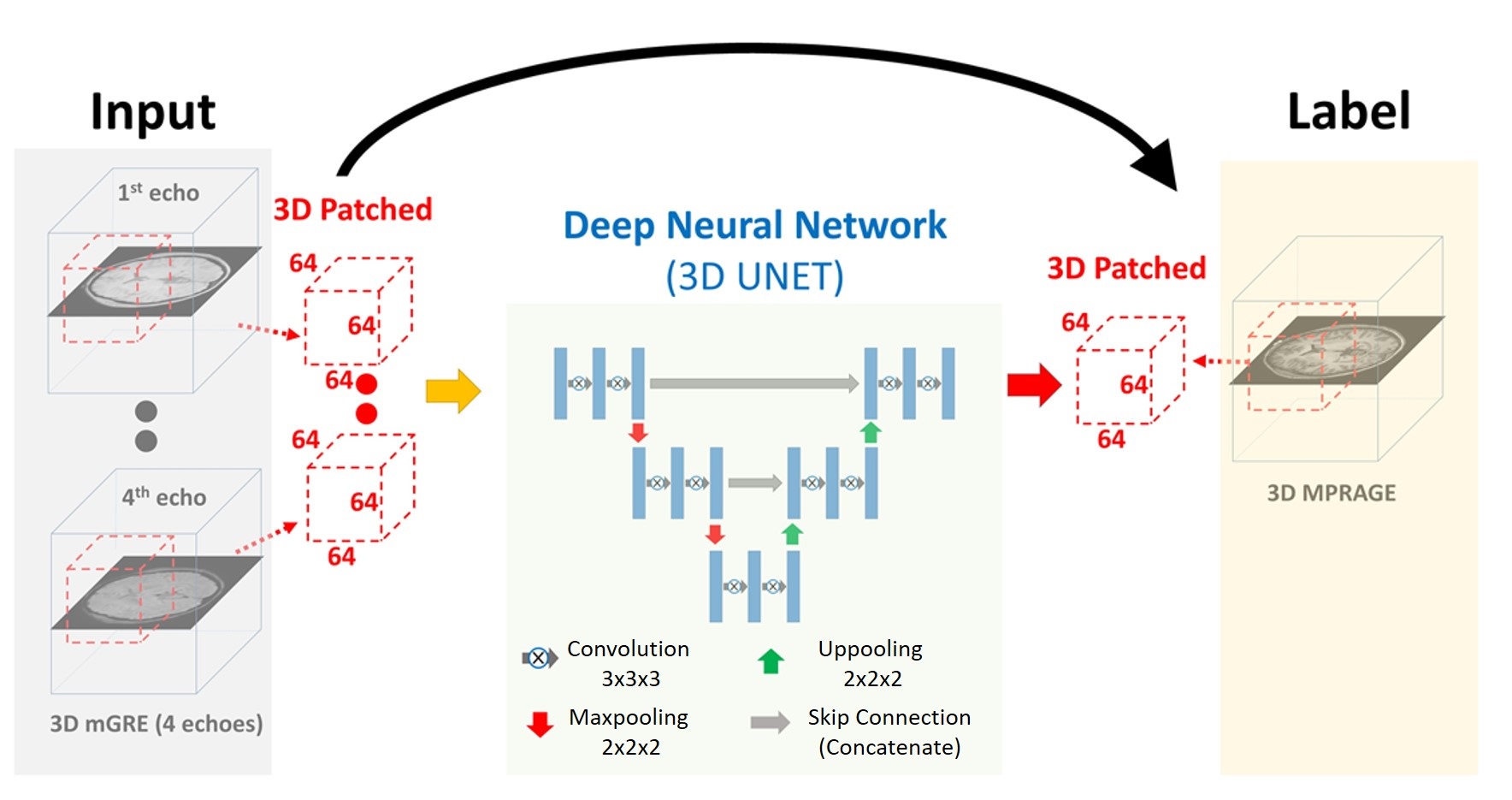
To make use of the 3D contextual information for voxel-wise estimation, a 3D version of U-NET [5,6] has been applied in this study. Detailed architecture of our network is demonstrated in Figure 1. Because of voxel size differences and possible displacements between the two sequences, mGRE images were registered to 1mm isotropic MPRAGE images using FLIRT in FSL [7]. Dataset were split by multiple patches with size of 64x64x64 to fit in the graphical processing unit (GPU). During testing, discontinuity of the patches were removed by allowing overlapping between the patches and averaging the overlapping regions. Learning was performed with mGRE and MPRAGE data obtained from 15 healthy subjects. Training and testing were carried out using TensorFlow on a system equipped with a single Nvidia GeForce GTX 1080ti GPU.
Validation
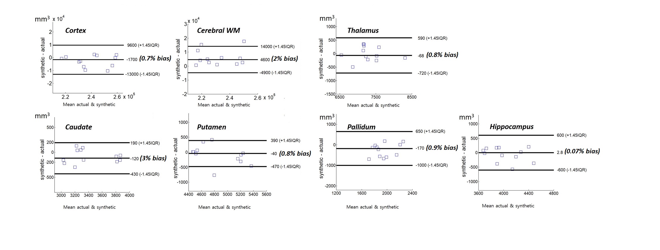
To evaluate the potential utility of the synthetic MPRAGE, volumetric analysis was conducted using the Freesurfer [8] for 6 healthy subjects not included in training set. From the automatically segmented regions, we compared the volumes of cortex, cerebral WM, putamen, pallidum, thalamus, caudate and hippocampus regions between the synthetic and the actual MPRAGE. A statistical comparison was performed using a paired t-test. Statistical significance was set at p<0.05. The bias relative to mean volume and variance of the two measurements (synthetic, actual) were calculated in the Bland-Altman plot. The regions in the left and right hemispheres were considered as independent in the procedure. For patient images, the performance was evaluated visually from the aspect of lesion assessment.
Results
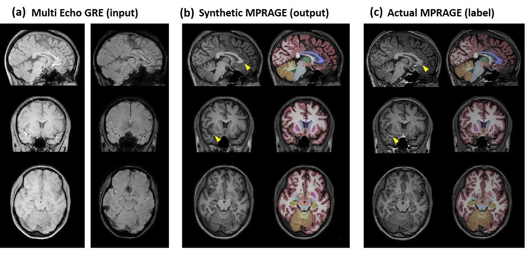
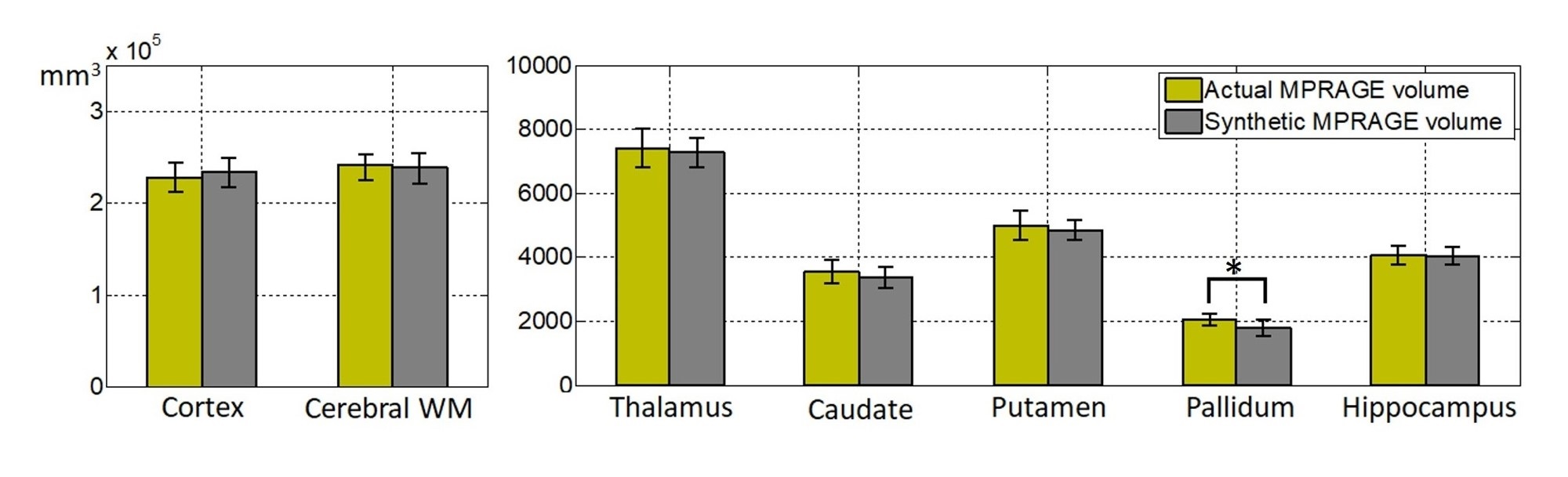
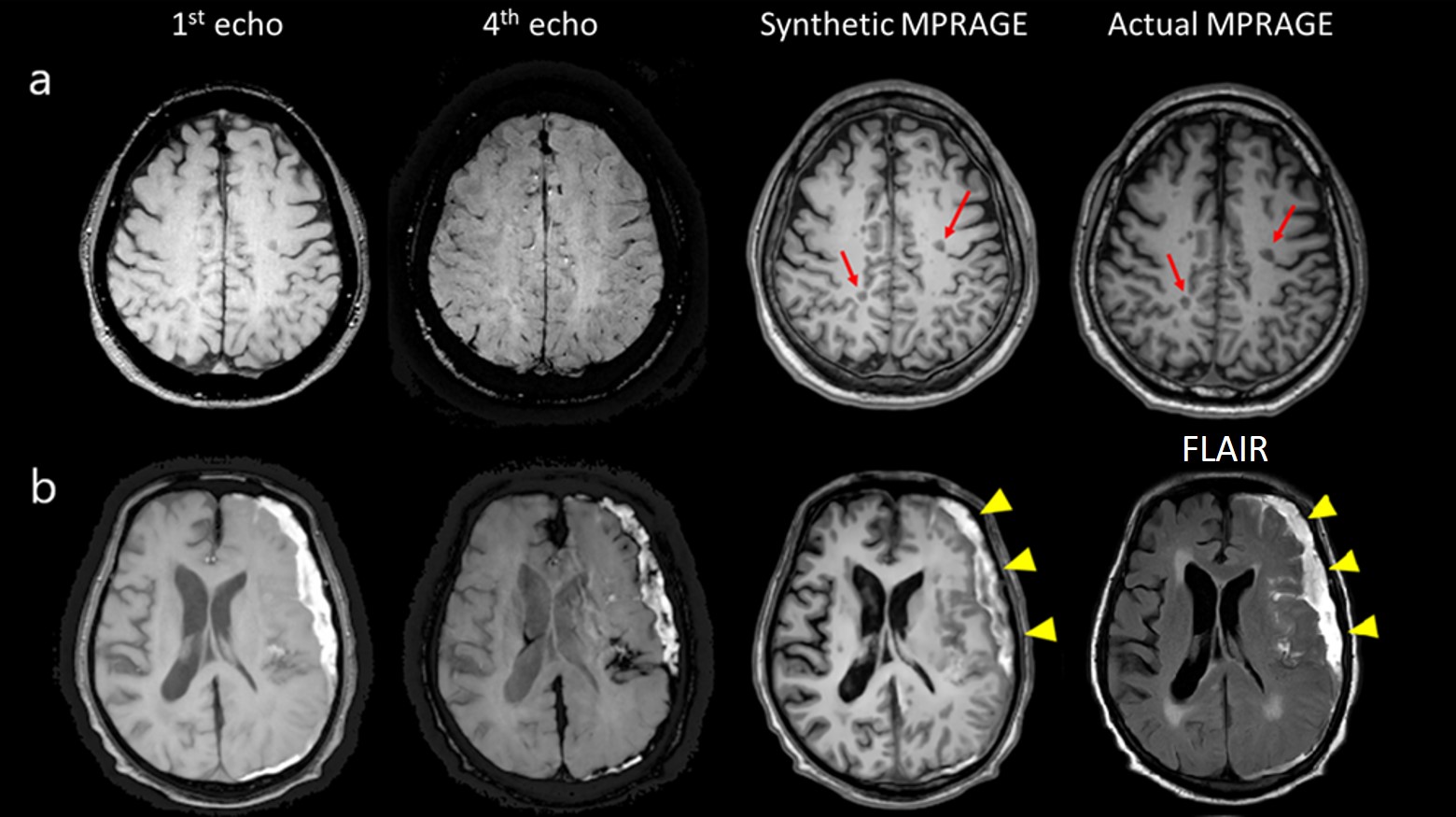
Figure 2 shows representative input, output (synthetic MPRAGE) and label (actual MPRAGE) images of the network. The segmentation results are also displayed. The synthetic images show overall similar contrast of WM/GM/CSF and subcortical structures although some regions are slightly blurred. Figure 3 shows the results of volumetric analysis. There was no statistically significant difference in the volumes measured by the two images in most regions except the pallidum (p=0.01). The biases of the measurements were less than 3% as shown in Fig. 4. In Figure 5, pathologic lesions are well visualized in the synthetic MPRAGE for both patients.
Discussion
We demonstrated successful generation of synthetic MPRAGE from mGRE by comparing the automatically measured volumes. The results of patient data show its ability to handle unlearned abnormal features, and their potentials for clinical use. There were some noticeable observations in the result. First, flow region (yellow marker) looks suppressed on the synthetic image. Second, slight underestimation of pallidum volume was observed. As this region is indefinite even in the actual MPRAGE, proper learning might have been difficult.Acknowledgements
This research was supported by Basic Science Research Program through the National Research Foundation of Korea(NRF) funded by the Ministry of Science, ICT and future Planning (NRF- 2016R1A2B3016273)
This research was supported by Graduate Student Scholarship Program funded by Hyundai Motor Chung Mong-Koo Foundation.
References
1. Haacke EM, Liu S, Buch S, Zheng W, Wu D, Ye Y. Quantitative susceptibility mapping: current status and future directions. Magnetic Resonance Imaging 2015;33:1–25.
2. Wang Y, Liu T. Quantitative susceptibility mapping (QSM): Decoding MRI data for a tissue magnetic biomarker. Magnetic Resonance in Medicine 2014;73:82–101.
3. Deoni SC , Rutt BK, Peters TM. Synthetic T1-weighted brain image generation with incorporated coil intensity correction using DESPOT1. Magnetic resonance imaging 2006;24(9):1241-1248.
4. Lorio S, Kherif F, Ruef A, Melie-Garcia L, Frackowiak R, Ashburner J, Helms G, Lutti A, Draganski B. Neurobiological origin of spurious brain morphological changes: A quantitative MRI study. Human brain mapping 2016;37(5):1801-1815.
5. O. Ronneberger PF, and T. Brox. U-net: Convolutional networks for biomedical image segmentation. arXiv:1505.04597 [cs.CV] 18 May 2015.
6. Lee D, Yoo J, Ye JC. Deep residual learning for compressed sensing MRI. 2017 18-21 April 2017. p 15-18.
7. Stephen M.Smith, et al. Advances in functional and structural MR image analysis and implementation as FSL. Neuroimage 2004;23(1):S208-S219.
8. Dale AM, Fischl B, Sereno MI. Cortical surface-based analysis. I. Segmentation and surface reconstruction. NeuroImage 1999;9(2):179-194.
Figures