3362
A Recurrent Inference Machine for accelerated MRI reconstruction at 7T1Institute for Informatics, University of Amsterdam, Amsterdam, Netherlands, 2Radiology, Academic Medical Center, Amsterdam, Netherlands, 3Spinoza Centre for Neuroimaging, Amsterdam, Netherlands
Synopsis
Accelerating high resolution brain imaging at 7T is needed to reach clinically feasible scanning times. Deep learning applies multi-layered neural networks as universal function approximators and is able to find its own compression implicitly. We propose a Recurrent Inference Machine (RIM) that is designed to be a general inverse problem solver. Its recurrent architecture can acquire great network depth, while still retaining a low number of parameters. The RIM outperforms compressed sensing in reconstructing 0.7mm brain data. On the reconstructed phase images, Quantitative Susceptibility Mapping can be performed.
Introduction
High resolution structural imaging of the brain at 7T is a timely procedure, that is difficult to endure for participants. In order to accelerate imaging, k-space can be incoherently undersampled beyond the Nyquist criterion. Compressed sensing (CS) reconstructs images using a predefined transform such as the Wavelet transform. Deep learning applies multi-layered neural networks as universal function approximators and is able to find its own compression implicitly. This allows to further accelerate image acquisition. Here we propose a Recurrent Inference Machine$$$^1$$$ (RIM) that is designed to be a general inverse problem solver. Its recurrent architecture can acquire great network depth, while still retaining a low number of parameters.Methods
The main network architecture is summarized in Figure 1. The RIM uses an update function $$$h_{\phi}$$$ over a series of $$$T$$$ time-steps. For each time-step $$$t$$$, the update function takes the current best estimate $$$\mathbf x$$$ of the true MR-image and outputs an incremental update $$$\Delta\mathbf x_t$$$ to take in image space in order to reach the next and improved estimate $$$\mathbf x_{t+1}=\mathbf{x_t}+\Delta\mathbf{x_t}$$$. Convolutional layers help the RIM extract features from correlating neighbour-pixels, while intermediate gated recurrent units (GRU) maintain the RIM’s latent states as reconstruction progresses through time and network depth. Once processed and activated, these states are used as gates in $$$1\times 1$$$-convolutions to help recombine the extracted features in a meaningful manner. To further aid the network in finding meaningful feature transformations, it is guided by the log-likelihood gradient from the posterior distribution as another input to $$$h_{\phi}$$$, while the more elusive prior distribution is meant to be learned internally by the network’s parameters $$$\phi$$$.
The RIM was implemented for both real- and complex-valued parameters, through the use of standard calculus and Wirtinger-calculus, respectively. The complex-valued network used a cardioid activation function$$$^2$$$, while ReLUs were used on the real-valued network. The MSE averaged over all time-steps $$$T$$$ was used as the learning objective of the network. It was trained on a range of acceleration factors (ranging from two-fold to six-fold), using sub-sampling patterns randomly generated from gaussian kernels, in order to generalize well to a large range of corruption processes.The $$$l_2$$$-norm was used as a loss function.
To study the network depth, the RIM was trained for 8 time-steps and losses were compared between networks using real- and complex-valued parameters. Training was performed on patches of 30x30 voxels, yielding 12,050 iterations over 18 epochs.
Data was acquired of two healthy subjects on a Philips 7T scanner (Philips,The Netherlands), comprising of 3D multi-echo FLASH data series of two healthy subjects with FOV 224x224x126 mm, resolution 0.7mm$$$^3$$$, TR/TE=23.4/3-21 ms, 6 echoes, FA 12$$$^o$$$, fully sampled with elliptical shutter, scanning time 22 minutes.The RIM was trained and tested on data of one subject, while the other subject’s data was used a hold out set for evaluation.
CS reconstruction was performed using the Berkeley Advanced Reconstruction toolbox, with ESPIRiT auto calibration$$$^3$$$, an l1-norm sparsity term using the wavelet transform, and optimized regularization.
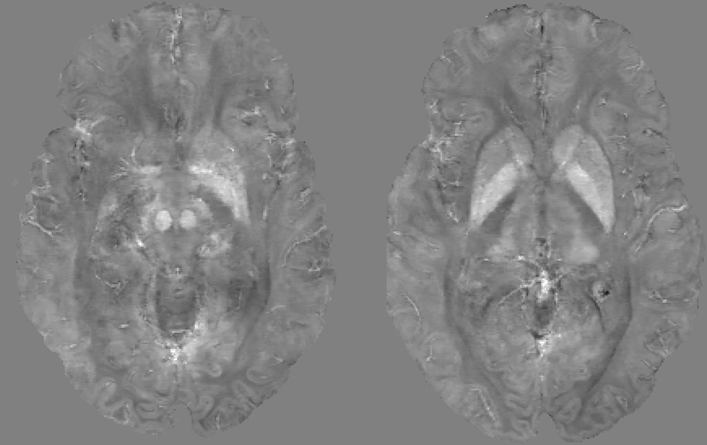
A Quantitative Susceptibility Map (QSM) was obtained from one TE (TE$$$_5$$$) using STISuite$$$^4$$$.
Results
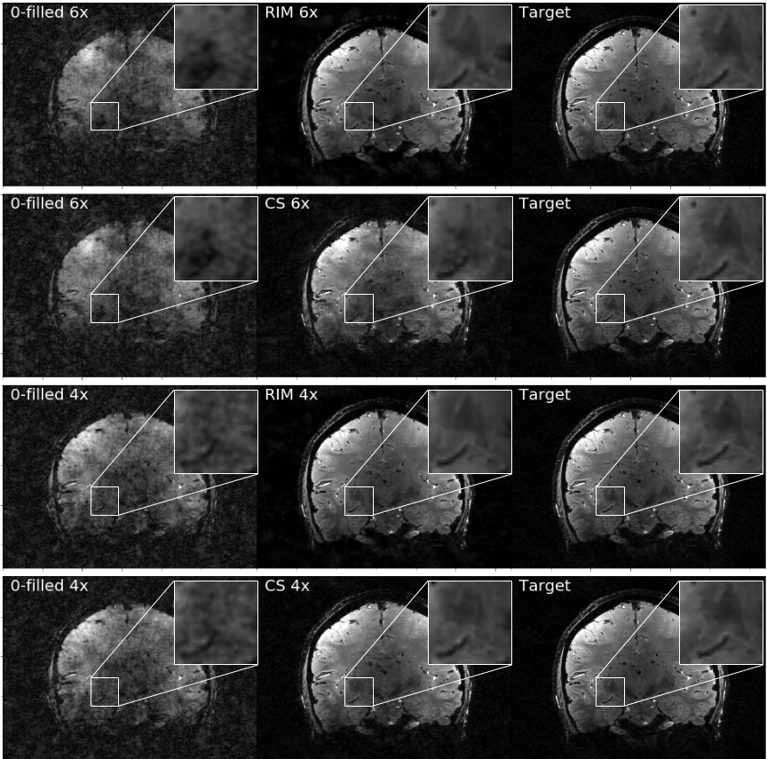
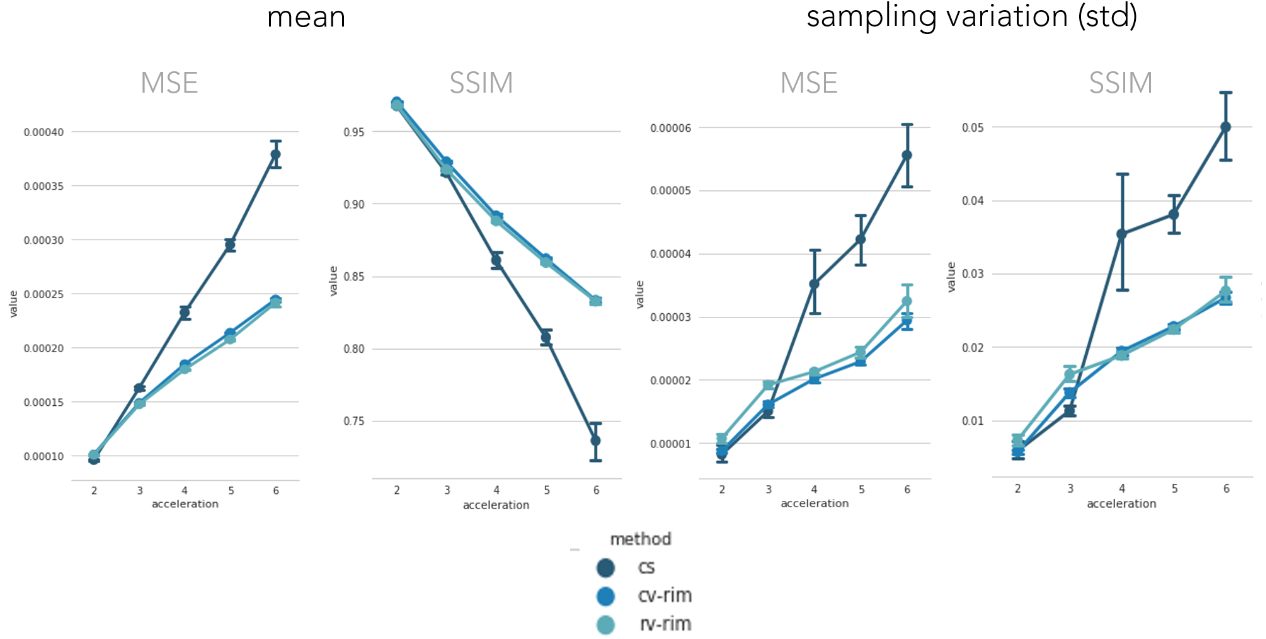
Training took 20 hours on a single GPU-card. Inference times ranged around 500 ms. Figure 2 illustrates the network loss on the evaluation set. The heatmap shows loss as a function of training iterations and recurrent timesteps of the RIM, while the loss curves for the real- and complex-valued networks at 4-fold and 6-fold acceleration are illustrated for the 10th time-step (2 more than what was trained on). Real- and complex-valued RIMs perform similarly, but better than CS.Figure 3 shows sample reconstruction magnitude images. The Mean Squared Error (MSE) and Structural Similarity (SSIM) of reconstructed images relative to the target is given in Figure 4. Figure 5 shows QSM-results on processed phase images.Discussion
Our recurrent inference machine (RIM) was trained on data of a range of echo times and acceleration factors. Training on a single subject’s data already sufficed to outperform CS on unseen data. Furthermore, the RIM was more invariant to the subsampling pattern. Future work will involve training on larger datasets.
To optimize image reconstruction time, a trade-off needs to be found between the network depth, i.e. the number of timesteps and reconstruction accuracy. The fact that a lower loss was obtained for 8 compared to 15 timesteps, means that a time-efficient network with few recurrent iterations can be used.
Conclusion
A Recurrent Inference Machine (RIM) can reconstruct accelerated high resolution magnitude and phase data acquired at 7T. The network was trained on a range of TEs and acceleration factors, outperforms CS and is efficient at inference time.Acknowledgements
No acknowledgement found.References
1. Putzky P, Welling M. Recurrent Inference Machines for Solving Inverse Problems. arXiv:1706.04008, 2017.
2. Virtue P, Yu SX, Lustig M. Better than Real: Complex-valued Neural Nets for MRI Fingerprinting. arXIV:1707.00070v1, 2017.
3. Uecker M, Lai P, Murphy MJ, Virtue P, Elad M, Pauly JM, Vasanawala SS, Lustig M. ESPIRiT — An Eigenvalue Approach to Autocalibrating Parallel MRI : Where SENSE Meets GRAPPA. Magn. Reson. Med. 2014;1001:990–1001.
4. Liu C, Li W, Tong K a., Yeom KW, Kuzminski S. Susceptibility-weighted imaging and quantitative susceptibility mapping in the brain. J. Magn. Reson. Imaging 2015,23-41.
Figures
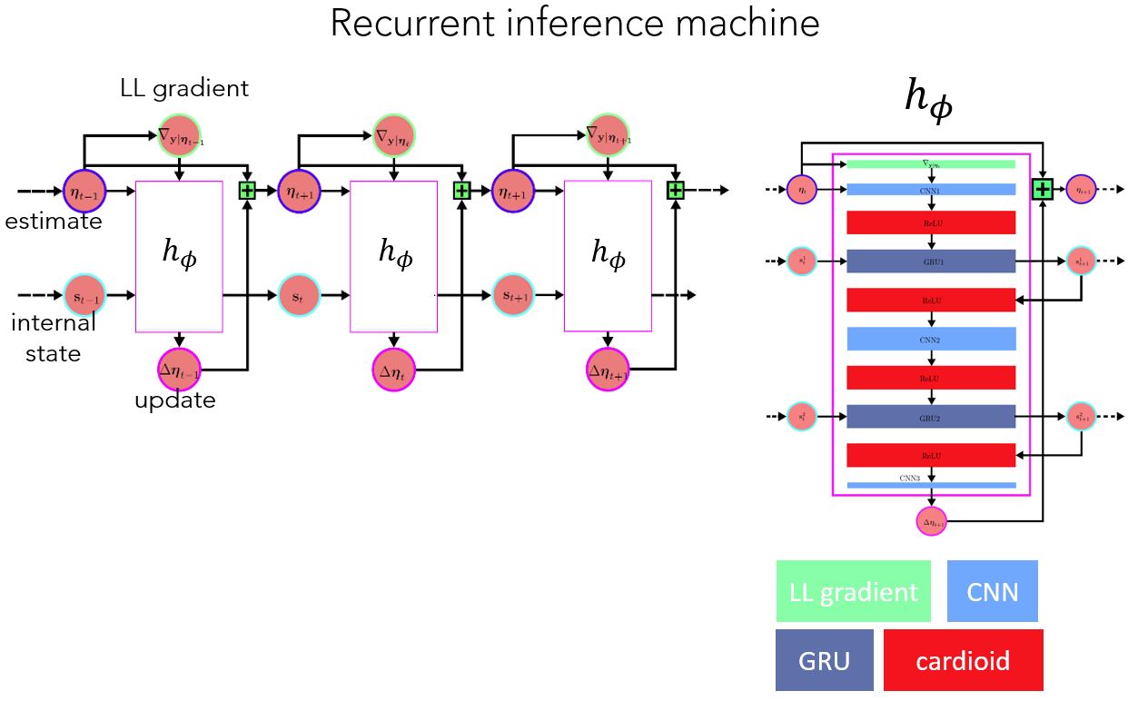
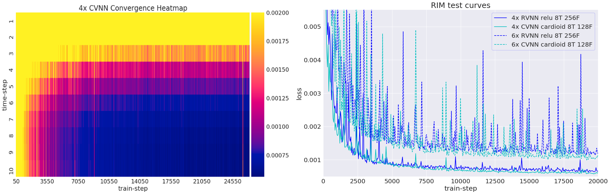
Figure 2. Left: Training loss over time-steps and training iterations (train-steps), illustrating improved performance over recurring time steps, and convergence during training.
Right: training curves, showing the loss function over multiple training iterations. The complex- and real-valued networks perform similarly, both for 4-fold and 6-fold acceleration. 8T: 8 time steps. 128/256F: number of Features.