Synopsis

Inclusion of voxels containing CSF and/or blood vessels can bias ROI statistics used in DSC-MRI analysis. In order to address this problem we propose an automatic method for tissue segmentation based on hemodynamic features obtained from DSC-MRI data. Application of the method in test subjects shows promising results.

Introduction

Dynamic susceptibility contrast (DSC) MRI can be used to characterize the microvasculature of the brain. A commonly used analysis approach is to extract a summary statistic from a region of interest (ROI) in the brain. However, if voxels containing other tissue types such as cerebrospinal fluid (CSF) or blood vessels are included in the ROI, the statistic will be biased. A segmentation that identifies voxels of unwanted tissue types would thus be beneficial. Furthermore, the segmentation should ideally be based on images already included in the examination to reduce examination time.

A segmentation method using the DSC data itself for identification of CSF voxels has been proposed by Kao et al¹. In this study, that method is extended to also identify vessels by addition of another feature extracted from the DSC data in combination with regularized clustering.

Methods

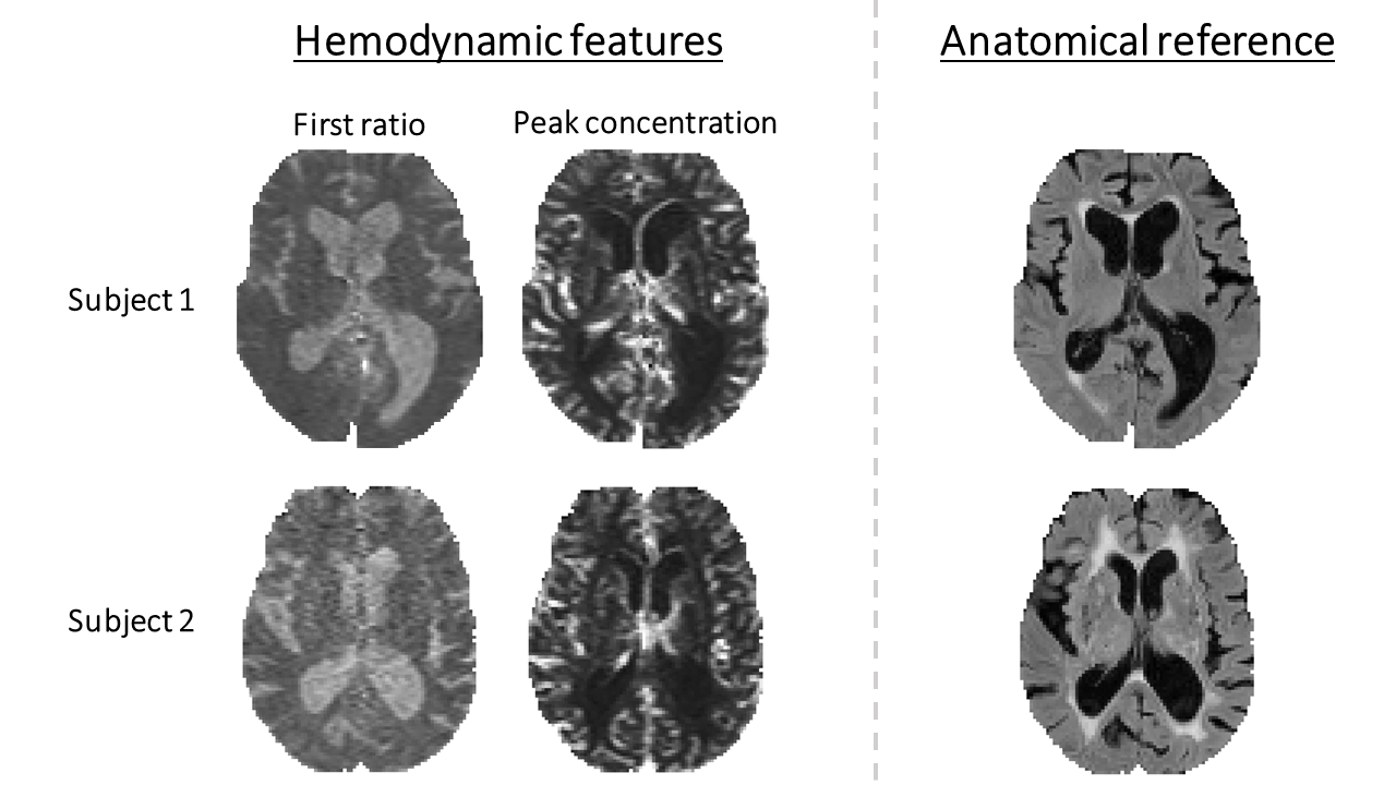
The method for identification of CSF voxels proposed by Kao et al. exploits the long T1 of CSF and the fact that steady state has not been reached during the first dynamics¹. The feature, called “first ratio” (FR), is the signal at the first dynamic normalized to some reference. In this study, FR was calculated as

$$FR=\frac{S(1)}{S_0}$$

where S(t) is the signal at the t^th dynamic and S₀ is the average signal at steady state before contrast agent injection, i.e. during baseline.

Vessels can be assumed to differentiate from other tissue types by having a higher increase in contrast agent concentration after injection. To capture this characteristic, a feature based on the peak concentration (PC) is proposed, calculated as

$$PC=\frac{1}{3} \sum^{T_p+1}_{t=T_p-1}C(t)$$

where C(t) is the contrast agent concentration at the t^th dynamic and Tp is the dynamic with maximum C(t), i.e. the peak concentration. Conversion from signal to concentration was performed according to

$$C(t)=-\frac{1}{TE}\ln\frac{S(t)}{S_0}$$

where TE is the echo time.

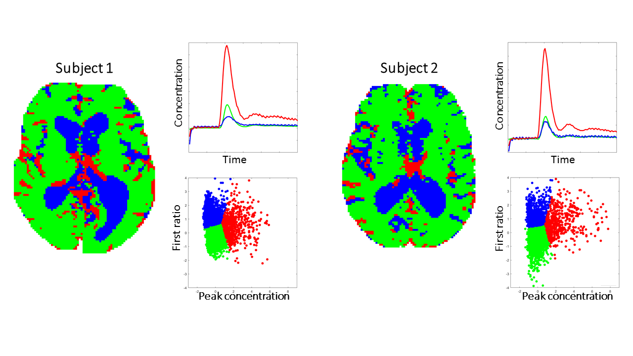
The k-means algorithm² was used to cluster voxels into three clusters corresponding to CSF, vessels and brain parenchyma. To improve interpretability and robustness of the clustering, a regularization term was added to the k-means objective function

$$J(\mu_k)=\sum_k\left(\sum_{x\in A_k}||x-\mu_k||^2+\lambda_k||\mu_k-\mu_{0,k}||^2\right)$$

where x is the feature vector of a voxel, A_k is the set of voxels in the k^th cluster, μ_k is the center of the k^th cluster and μ_0,k is the center of the k^th cluster proposed prior to the optimization. λ_k are regularization factors calculated as

$$\lambda_k=\frac{\sum_k\sum_{x\in A_{0,k}}1}{\sum_k\sum_{x\in A_k}1} $$

where A_0,k is the set of voxels in the k^th cluster proposed prior to the optimization.

A_0,k and μ_0,k were estimated separately for the CSF and vessel classes. For the CSF prior class, Otsu thresholding³ of the FR feature was used¹. Furthermore, connected components (4-connectivity) containing fewer than 10 voxels were excluded from the class. For the vessel prior class the 10 % voxels with highest PC value was chosen. Voxels assigned to both the CSF and the vessel prior classes were excluded. Voxels not included in neither the CSF nor the vessel class were assigned to the brain parenchyma class followed by the same connected component reduction step as for the CSF class. Some voxels were thus not necessarily included in any of the prior sets A_0,k. All processing was done using MATLAB.

To study the usefulness of the proposed method, MR images of two idiopathic normal pressure hydrocephalus patients were acquired with a 1.5T Philips Gyroscan Intera. For anatomical reference FLAIR images were acquired (voxel size 1.2×1.2×3mm³). DSC-MR images were obtained every 1000ms with GE-EPI (voxel size 1.8×1.8×5mm³). A bolus (5ml/s) of 0.1mmol/kg body weight Gd-DTPA (Schering, Magnevist 0.5mmol/ml) was initiated at the tenth dynamic into the right antecubital vein. Skullstripping was employed to form an ROI encompassing the brain. For each subject, all voxels within the ROI were extracted and clustered using the described method. Before clustering, features were normalized to have zero mean and unit variance.

Results

Conclusion

Acknowledgements

References

1. Kao YH, Teng MMH, Zheng WY, Chang FC, Chen YF. Removal of CSF pixels on brain MR perfusion images using first several images and Otsu’s thresholding technique. Magn Reson Med 2010;64:743–748.
2. Macqueen J. Some methods for classification and analysis of multivariate observations. Proc Fifth Berkeley Symp Math Stat Probab 1967;1:281–297.
3. Otsu N. A Threshold Selection Method from Gray-Level Histograms. IEEE Trans Syst Man Cybern 1979;9:62–66.