3232
Characterization of Diffusion Metric Map Similarity in MRI Data from a Clinical PACS using the Histogram Distance1Radiology, Massachusetts General Hospital, Boston, MA, United States, 2Radiology, Harvard Medical School, Boston, MA, United States
Synopsis
As data reuse becomes more popular, it is critical to develop methods that characterize the similarity of data. Methods have been developed that characterize raw image files, but users often only have access to calculated parameter maps. Here we describe a histogram-distance-based method applied to diffusion metric maps generated from MRI data extracted from a clinical data repository. We find that metric maps from GE scanners are less similar than that from Siemens scanners. We also find within vendor differences at any selection of the acquisition parameters considered here (field strength, number of gradient directions, b-value and vendor).
Introduction
Data reuse can aid in the development of 1)processing and analysis methods, 2)treatments for rare diseases, and 3)tools for the characterization of scanner reproducibility1. However, a general problem in data reuse is whether the data are similar enough to be meaningfully combined. Previously2, we have applied a histogram-distance-based method to diffusion-metric maps that arose from a multi-site study, acquired using a harmonized imaging protocol. In this study, we apply this method to diffusion MRI brain data originating from a repository of clinical MRI images. Here, the imaging protocol may vary by presented symptom, by imaging department, and over time, all of which presents particular challenges to data reuse. The goal this work is to use this method to characterize the similarity within and between collections of calculated parameter maps.Methods
This study was approved by the Partners Human Research Committee and subjects granted their written informed consent. We obtained radiology reports from patients who underwent brain MRI scans, but who were ultimately free of any pathology, by querying the Partners Research Patient Data Registry3 (RPDR) clinical database via a query by age and diagnosis. The age range was 18-54 and the diagnosis selection was terms specific to migraines. We used natural language processing to filter the resulting reports to exclude those with any affirmative mention of pathology or artifacts. The filtration resulted in 1,266 usable diffusion-weighted MRI data sets. We then eddy- and motion-corrected each volume within each diffusion data set using FSL’s (FMRIB, Oxford, UK) eddy_correct tool and the gradient direction vectors were corrected for the observed motion. Calculation of fractional anisotropy (FA) and mean diffusivity (MD) was then performed using FSL’s dtifit tool. Histograms of FA and MD values were constructed. Each histogram was calculated using 100 bins with ranges (0.0-1.0] for FA and (0.0-0.004] mm2/s for MD. The b-values, number of gradient directions, scanner vendor, and field strength were recorded for each histogram. The histogram distance was calculated both within and between groups using the Hellinger4 metric, which was selected based on our previous study. The following comparisons were performed (if a specific tag value is not noted, no restriction is set on its value): 1) within vendor (Siemens, GE), 2) between vendor (Siemens versus GE), 3) between vendor, b=1000 s/mm2, 4) within Siemens, b=1000 s/mm2 versus b=700 s/mm2, 5) within Siemens, field strength (1.5T versus 3.0T), 6) between vendor, b=1000 s/mm2, 30 gradient directions, 1.5T, 7) within Siemens, b=1000 s/mm2, 30 gradient directions, 1.5T versus 3.0T. Histograms of the histogram distance values were then generated.
We converted distance metric histograms into whisker plots with the whiskers extending 1.5 times the interquartile range past the third quartile. The Mann-Whitney U test, using all of the data points, was used to determine significance.
Results
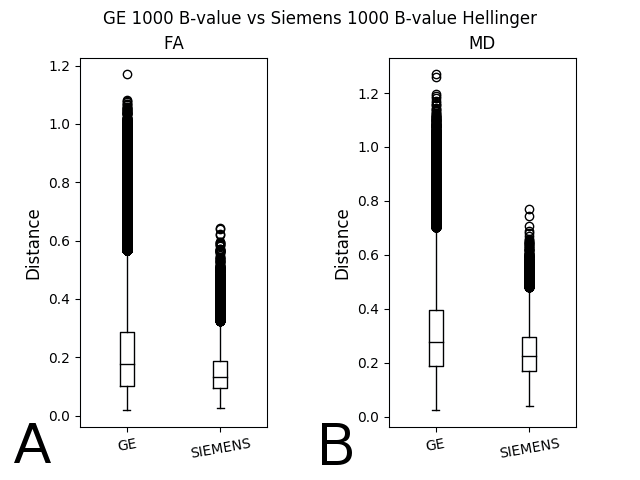
We present two of the above comparisons. Figure 1 shows the box-whisker plot of the Hellinger distance metric values for FA (1A) and MD (1B) for Siemens scanners versus GE scanners, b=1000 s/mm2. The differences in the histogram distance histograms were significant in both cases.
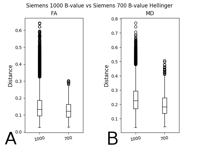
Figure 2 shows the box-whisker plot of the Hellinger distance metric values for FA (A) and MD (B) for Siemens scanners for b = 1000 vs 700 s/mm2. Again, the differences were significant in both cases.
Discussion
In Fig. 1 we see that the distribution of histogram distances for GE data is wider than it is for Siemens data. This difference was not explainable through differences in echo time, in-plane resolution, and slice thickness.
In Fig. 2 we looked within vendor at two different b-values and also saw significant differences between histogram-distance histograms. Again, these results were not explainable through differences in echo time, in-plane resolution, orslice thickness. One obvious reason for these results is the different pools of spins involved in the measurements, but these results give an indication of the magnitude of variability between the two b-values and the care that must be taken when combining data from different data sets.
Conclusions
Our results suggest that the FA and MD maps derived from diffusion data collected on GE scanners have a greater variability than those collected on Siemens scanners. This effect was observable both when comparing all GE data to all Siemens data, but also when comparing the two vendors while controlling for b-value, number of gradient directions, and field strength. We also found within-vendor differences. The results point to the careful curation necessary for the reuse of such data and show the utility of the method, which can also be used to detect poor quality data sets in a repository.Acknowledgements
We acknowledge assistance from the Massachusetts General Hospital RPDR team.References
1. J. B. Poline et al., "Data sharing in neuroimaging research," Front Neuroinform 6(9 (2012).
2. K. G. Helmer et al., "Multi-site Study of Diffusion Metric Variability: Characterizing the Effects of Site, Vendor, Field Strength, and Echo Time using the Histogram Distance," Proc SPIE Int Soc Opt Eng 9788 (2016).
3. R. Nalichowski et al., "Calculating the benefits of a Research Patient Data Repository," AMIA Annu Symp Proc, https://www.ncbi.nlm.nih.gov/pubmed/172386631044 (2006).
4. M. Deza, and E. Deza, Encyclopedia of Distances, Springer (2012).
Figures