Introduction

To study the venous vasculature in aging and disease, a normative venous vascular atlas of young healthy subjects against which populations can be compared would be beneficial. However, the creation of this atlas is far from trivial, and particularly challenging due to the variable venous architecture across individuals. Current efforts have focused on generating statistical maps of likely vessel location, rather than building explicit vascular maps¹. To avoid loss of information especially at the location of smaller vessels, we propose a novel atlasing method aimed at preserving details of the vascular anatomy while averaging across subjects. The atlas shows the average location and diameter of the venous vasculature in young and healthy brains. The deformation fields used to build the atlas can be used to explore the link between vessel location and diameter, and inter-subject variability.

Methods

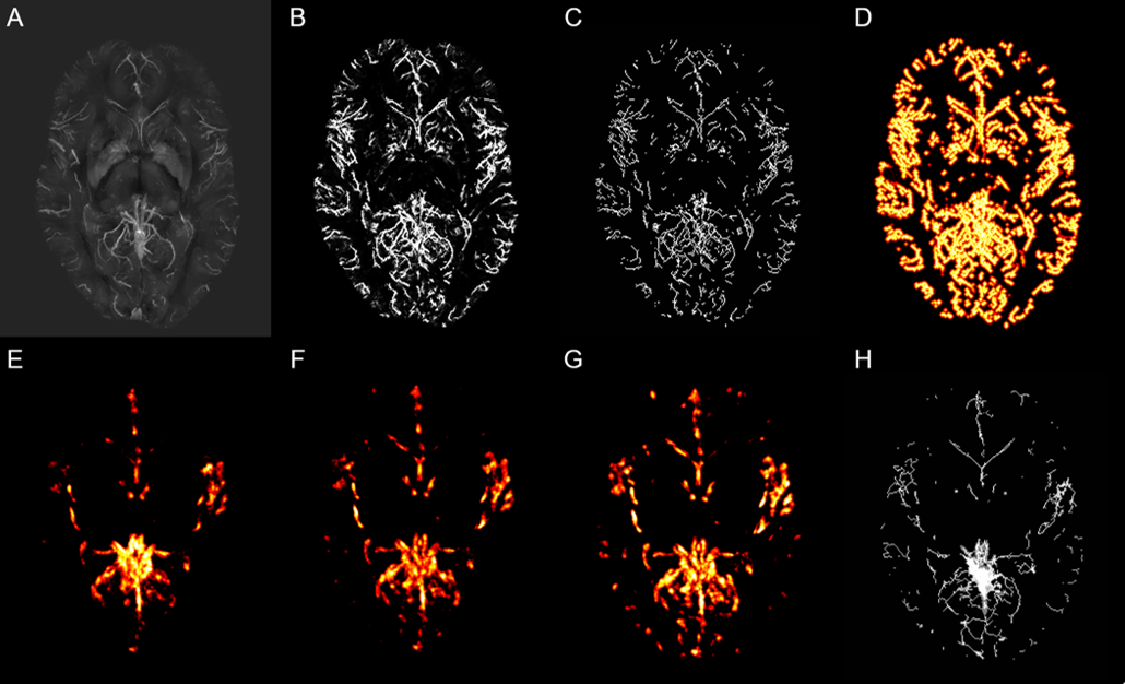
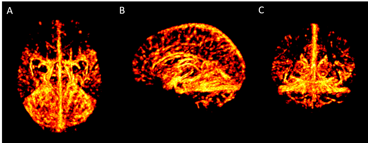
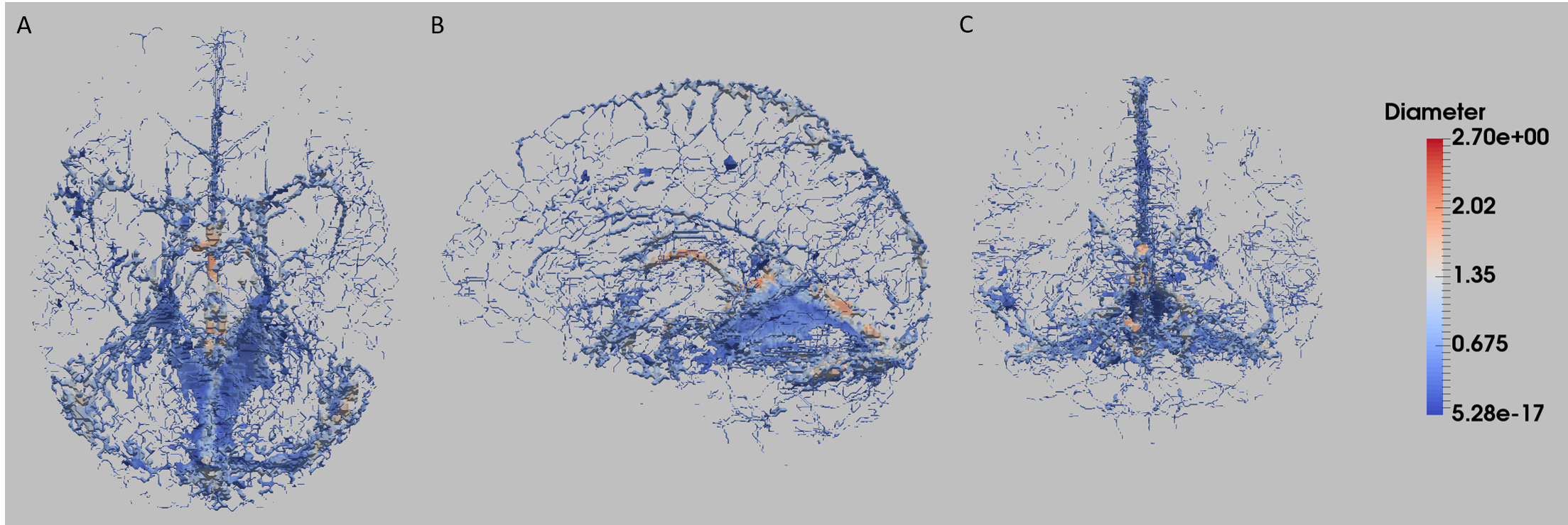
Sixteen healthy volunteers were scanned on a 7T Siemens MR system with flow compensation along all three axes at 0.6mm resolution with TR=23ms; TE=7.5ms; matrix = 320x320x104; GRAPPA acceleration R=3; and scan time=4min. Quantitative susceptibility mappings (QSM) were created using the Fast L1-Regularized QSM with Magnitude Weighting and SHARP background filtering toolbox² (Fig.1A). A multiscale vessel filter was applied on this QSM reconstruction to segment the venous vasculature. The filter estimates image edges recursively and uses a global probability diffusion scheme³ (Fig.1B). The vessel probability map and vessel diameter obtained from the vessel filter were then used in a three-step registration pipeline to create the atlas. To ensure an accurate registration a skeletonization algorithm adapted from ⁴ was applied on the probability maps (with a boundary and skeleton threshold=0.5) for each participant to reduce the vein to its centerline (Fig.1C). Due to the variability in vessel location across subjects the resulting centerline of the skeletonization algorithm was inflated to a 5mm, 15mm and 30mm radius by estimating a distance function truncated to the appropriate radius and mapped to [0,1] with highest values at the skeleton (Fig.1D). Groupwise registration of these inflated vessel maps was performed with the SyN algorithm of ANTs⁵. In a first step, participants were coarsely aligned to the participant closest to the average of the maps. The resulting deformation fields were also applied to each participant’s vessel diameter. The average of the level set probability and the diameter of all participants after the first registration was calculated (Fig.1E). These average images were used in the second pipeline as target images for the registration of the vessel location and the diameter. The average of the second pipeline was calculated (Fig.1F) and used as the new input for the third step of the registration pipeline (Fig.1G, Fig.2). In order to get back to the centerline of the average level set probability another skeletonization algorithm with a boundary threshold of 0.92-0.96 was applied. This centerline and the average diameter was used to get the partial voluming of the atlas (Fig.1H, Fig.3).

Results & Discussion

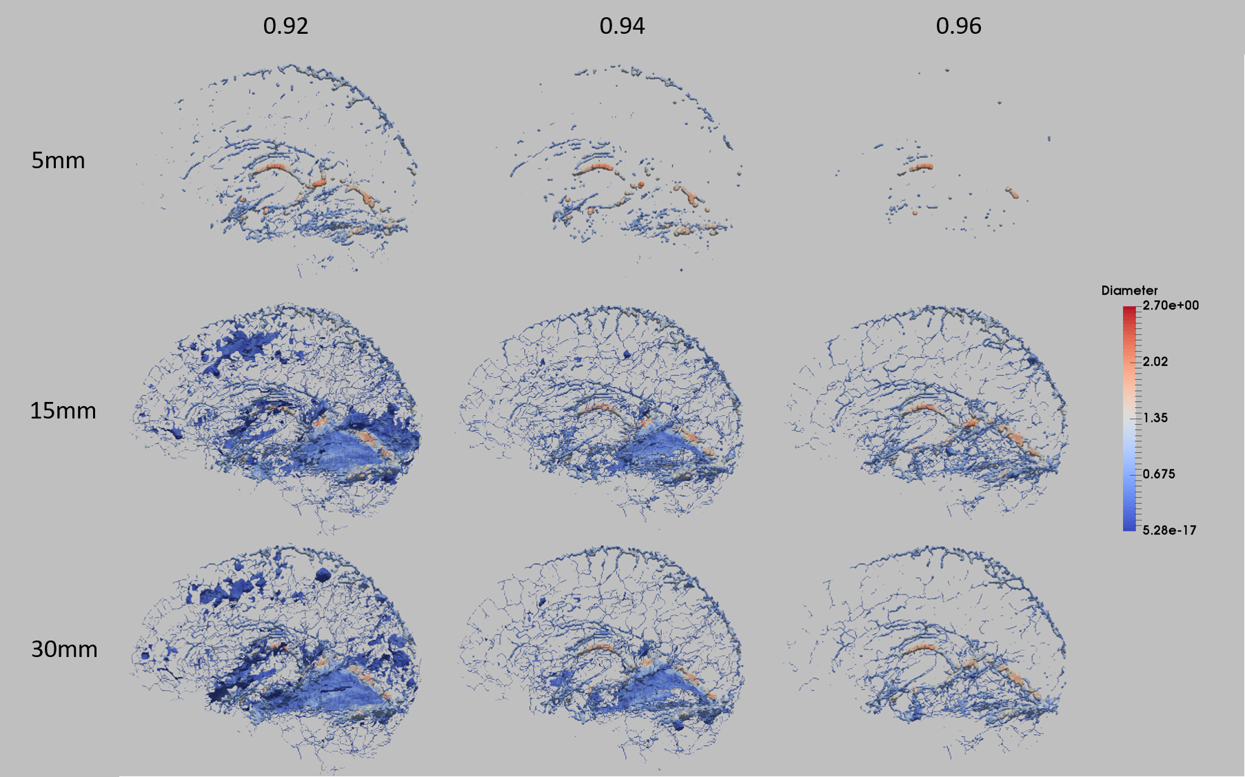
This three step registration method was successfully applied on the segmented venous vasculature with an inflation of the skeleton to create an atlas using QSM images. This atlas shows the average vessel location and diameter of sixteen healthy participants. In this framework, the inflation rate of the level set and the skeletonization parameters are the most important parameters for determining which vessels are included in the atlas (Fig.4). Overall, an inflation of 15 mm and a boundary threshold of 0.96 resulted in an atlas that best preserved the vasculature in the frontal lobe. However, due to the fact that the cerebellum anatomy is more similar across subjects and some sulci of the cerebellum are detected as vessels, this region appears denser in the atlas. Building an average of these inflated dense vessels leads to an overall high vessel probability in the vessel location average. Therefore, choosing a lower skeletonization parameter than the vessel probability in this region does not separate the vessels precisely. To solve the challenge of including the sparser vasculature in the frontal lobe and the dense vessels in the cerebellum different level sets and skeletonization parameters are required.

Conclusion

We proposed here a method for generating an atlas of the venous vasculature from QSM, which preserves fine details of the vascular tree. The resulting atlas depicts well the major veins of the brain, but also many smaller branches. As expected, there is significant spatial variability between regions and subjects, which may be explored from the estimated deformation fields. Future improvements will include defining region-specific thresholds to account for the variability in vessel detection, and further averaging steps better align the more variable cortical vessels.

Acknowledgements

The authors thank Domenica Wilfling and Elisabeth Wladimirov for their help with data acquisition and logistics. This work was supported by the Canadian National Sciences and Engineering Research Council (R0018142, RGPIN-2015-04665) and the Heart and Stroke Foundation of Canada (N.I.A. C.J.G.).