Synopsis

There is an increasing drive to use diffusion spectroscopy to infer the sizes of structures in samples. We present here the first use of the sine OGSE to infer the effective mean axon diameters in the human corpus callosum and study the effect on accuracy of reducing the number of images used in the inference. Aiming to reduce imaging times, this study examines how the number of frequencies or number of gradients affects accuracy and precision. We found that collecting OGSE data with two gradients gives a difference in results of less than 5% compared to six gradients.

Introduction

Methods

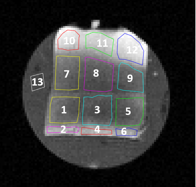
Sample A portion of normal-appearing corpus callosum from an autopsy human brain was obtained, which did not demonstrate any pathological changes. The sample was placed in agarose gel (2% w/v) within a 15 mL sample tube. MRI Images were acquired with a 2.5 cm diameter RF bird cage coil (Bruker Biospin), using a 7T Bruker Avance III NMR system (Paravision 5.0), with a BGA6 gradient insert (max strength: 430357 Hz/cm). 20 ms sine gradient pulses were used ranging from n=1 to 15 sinusodal waves (15 OGSE frequencies), with six gradient strengths used for each and separated by 24.52 ms. For n=1, g=(0, 22, 32, 39, 45, 50)% of g_max. For n=2-15, g=(0, 44, 61, 76, 88, 99)% of g_max. To our knowledge these correspond to the shortest effective diffusion times (0.5-7.5 ms) used on white matter. The following imaging parameters were used: NA=2, FOV=2.56 cm², matrix 64², TR=1250 ms, TE=50 ms. Analysis The mean ± standard deviation of the signal in the ROIs (Figure 1) was calculated. The signal was assumed to be described by a two compartment model of the form,

$$ E(\omega=2\pi n/\sigma,g) = (1-f_{axon})e^{-bD_{h}} + f_{axon}e^{-\beta(D_{i},AxD)}$$

where f_axon is the axon packing fraction, D_i is the intra-axonal diffusion coefficient, D_h is the hindered diffusion coefficient, and AxD is the effective mean axon diameter⁸. Signals were fitted to the two compartment model using least squares minimization to extract AxD. Higher OGSE frequencies were then removed and the remaining data was refit to the model to see how fitted parameters changed to determine if certain images could be excluded from data collection in clinical settings. Model fitting was also repeated using all possible combinations of the gradient strengths.

Results

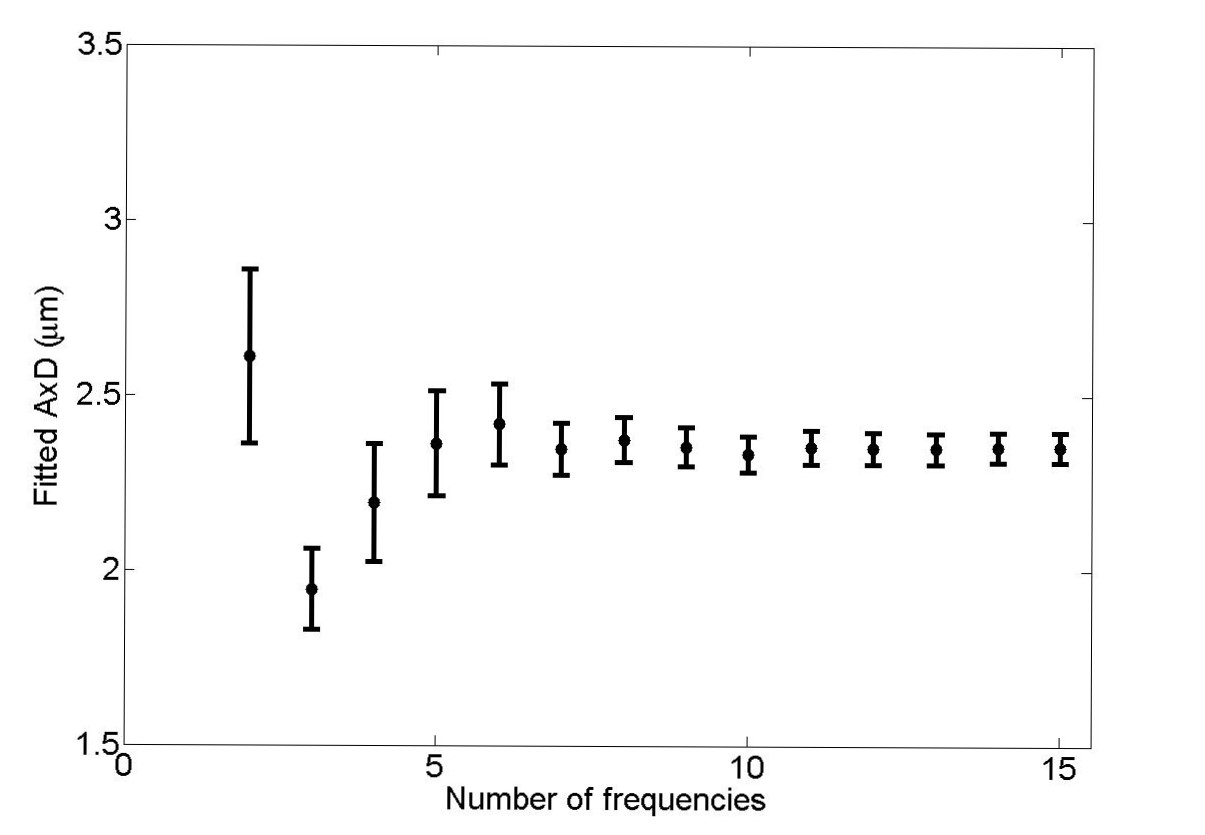
Figure 2 shows the variation in fitted AxD as a function of number of frequencies. Between 7 and 15 frequencies, AxD are within 1% of each other. The highest and lowest AxD occur when using 2 or 3 frequencies. The smallest fitted AxD is 1.9 ± 0.1 um (3 frequencies). The highest fitted AxD is 2.6 ± 0.2 µm (2 frequencies). Compared to AxD with 15 frequencies, these are respective differences of 17% and 3%. Error decreases when more frequencies are used.

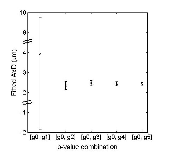
Figure 3 shows variation in fitted AxD when using only two gradient strengths. With the exception of the first gradient, fitted AxD are within 5% of each other. The error also increases when smaller gradients are used, with fitted AxD values ranging from 2.40 ± 0.08 µm with the highest gradient strength to 4 ± 6 µm with the smallest gradient strength.

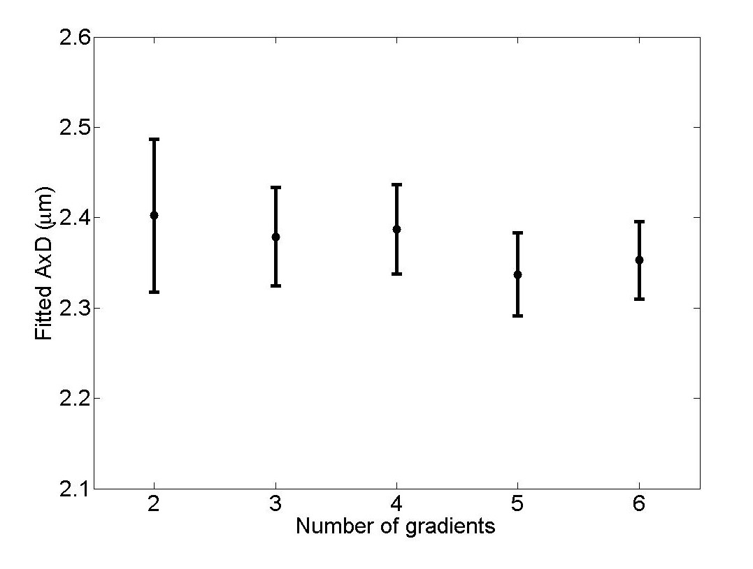
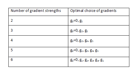
Figure 4 shows fitted AxD for the best combinations with each number of gradients (these combinations are shown in Table 1). The fitted values in Figure 4 are all within 3% of each other, while error when using just two gradients is about 2 times larger than when using all six gradients.

Discussion and Conclusion

Acknowledgements

References