3107

More certainty about your uncertainty in diffusion MRI microstructure estimates

Robbert Leonard Harms¹ and Alard Roebroeck¹

¹Department of Cognitive Neuroscience, Maastricht University, Maastricht, Netherlands

Synopsis

Diffusion MRI microstructure approaches use point estimates ignoring the uncertainty in these estimates. In this work, we evaluate two general methods to quantify uncertainty and generate uncertainty maps for any microstructure model. We find that the Fisher Information Matrix method based in nonlinear optimization is fast and accurate for models with few parameters. The Markov Chain Monte Carlo (MCMC) based method takes more time, but provides robust uncertainty estimates even for sophisticated models with more parameters. Uncertainty estimates of microstructure measures can help power evaluations for group/population studies and assist in data quality control and analysis of microstructure model fit.

Introduction

Biophysical compartment microstructure models in diffusion MRI (dMRI) promise greater specificity over Diffusion Tensor Imaging (DTI) and offer additional microstructure measures such as axonal density, dispersion and diameter distributions. Models of this type include (but are not limited to) CHARMED¹⁠, NODDI^2⁠, AxCaliber^3⁠, ActiveAx⁴⁠ and variations. Almost invariably, diffusion MRI microstructure approaches use point estimates for all inferences on differences between brain locations, tracts and patient groups. However, not every point estimate has equal confidence and this uncertainty is mostly ignored in diffusion microstructure studies. Although the uncertainty of DTI parameters^5,6⁠, and some fiber orientation models^7-9⁠ has been discussed, very little development in the quantification of uncertainty in diffusion MRI microstructure estimates has taken place. A simple but essential measure of uncertainty is provided by the covariance matrix of the parameter estimates, where the square root of the diagonal entries provide the individual parameter uncertainties as standard deviations. In this work, we explore two general methods for approximating such a covariance matrix for any microstructure model and generate uncertainty maps: one based in nonlinear optimization and one based in Markov Chain Monte Carlo (MCMC) sampling.

Methods

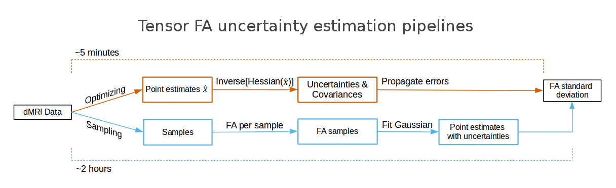
The first method for approximating the parameter covariance matrix is by using the Fisher Information Matrix (FIM) evaluated at a point estimate obtained from nonlinear optimization. The inverse of the FIM, where the FIM can be computed as the Hessian (the matrix of all second partial derivatives), represents, in the limit of high signal-to-noise ratio, the parameter covariance around the optimized point estimate. The second method approximating the parameter covariance matrix can be computed by fitting a multivariate distribution to the samples obtained by MCMC sampling. Here we consider a multivariate Gaussian distribution. Moreover, under flat uninformative priors, which we consider here, the sampling posterior approximates the likelihood. Under these assumptions, the Gaussian fit to the sampled posterior gives a new point estimate (the posterior mean) and a covariance around that mean, whereas the optimized point estimate approximates the posterior mode and the FIM gives the covariance around that mode. In theory, the covariance matrices given by the optimization and sampling method are only equal if the posterior density is symmetric and unimodal, since then the mode and mean are equal. While sampling provides easy access to uncertainties of measures derived from estimated parameters, for example Fractional Anisotropy (FA), Mean Diffusivity (MD) and Neurite Density Index (NDI), error propagation can provide the same information from the optimized point estimate with the FIM. Figure 1 illustrates uncertainty estimation for derived measures using sampling and using error propagation.

Results and discussion

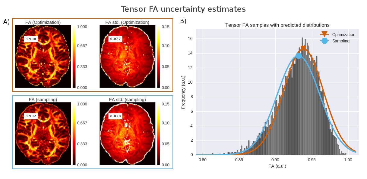
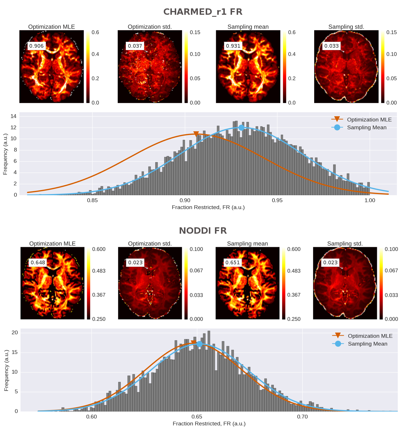
To illustrate the difference in the optimization and sampling based uncertainty methods, we optimized and sampled three models, CHARMED_r1 (with 1 restricted intra-axonal compartment) NODDI and Tensor, to a dataset of the HCP MGH Consortium (dataset 1003). This dataset was acquired at a resolution of 1.5mm isotropic with 4 shells of b=1000, 3000, 5000, 10,000, s/mm^2, with respectively 64, 64, 128, 256 directions and with 40 b0 volumes. Optimization and sampling where performed using the standard analysis pipelines in the Maastricht Diffusion Toolbox (MDT; https://github.com/cbclab/). Figure 1 shows a comparison for DTI FA (on the b=1000 shell) between the point estimates and the corresponding standard deviations computed using the two methods. It can be seen that uncertainty increases significantly towards the middle of the brain, correlating to the lower SNR further away from RF receive coils, whereas both methods provide similar results. Figure 2 shows a comparison between the two uncertainty methods for both the CHARMED_r1 and the NODDI model. Again there is close correspondence between between the two uncertainty methods for NODDI, but a superior result for the sampling method for CHARMED_r1.

Conclusion

In this work we compared two methods for computing uncertainties around parameter estimates, an optimization method and a sampling method. Although some derived indices, such as FA, have skewed distributions, most sampled microstructure parameter distributions are close to Gaussian, justifying the Gaussian fit in the sampling method for uncertainties. For models with low number of parameters, such as the NODDI and Tensor model, we recommend the optimization method with the FIM due to the (relative) speed of processing and accuracy compared to the sampling method. For models with higher number of parameters, such as CHARMED, we recommend the sampling method method for uncertainty, given its robustness. Robust and accurate estimates of uncertainty of microstructure measures can help power evaluations for group and population studies and play an important role in data quality control and analysis of microstructure model fit.

Acknowledgements

The research was supported by the Netherlands Organization for Scientific Research (NWO) VIDI 14637 (AR), and the European Research Council Starting Grant, MULTICONNECT #639938 (RH, AR).

References

1. Assaf Y, Basser PJ. Composite hindered and restricted model of diffusion (CHARMED) MR imaging of the human brain. Neuroimage. 2005;27(1):48-58. doi:10.1016/j.neuroimage.2005.03.042.

2. Zhang H, Schneider T, Wheeler-Kingshott CA, Alexander DC. NODDI: Practical in vivo neurite orientation dispersion and density imaging of the human brain. Neuroimage. 2012;61(4):1000-1016. doi:10.1016/j.neuroimage.2012.03.072.

3. Assaf Y, Blumenfeld-Katzir T, Yovel Y, Basser PJ. AxCaliber: A method for measuring axon diameter distribution from diffusion MRI. Magn Reson Med. 2008;59(6):1347-1354. doi:10.1002/mrm.21577.

4. Alexander DC, Hubbard PL, Hall MG, et al. Orientationally invariant indices of axon diameter and density from diffusion MRI. Neuroimage. 2010;52(4):1374-1389. doi:10.1016/j.neuroimage.2010.05.043.

5. Jones DK. Determining and visualizing uncertainty in estimates of fiber orientation from diffusion tensor MRI. Magn Reson Med. 2003;49(1):7-12. doi:10.1002/mrm.10331.

6. Jones DK, Basser PJ. “Squashing peanuts and smashing pumpkins”: How noise distorts diffusion-weighted MR data. Magn Reson Med. 2004;52(5):979-993. doi:10.1002/mrm.20283.

7. Behrens TEJ, Woolrich MW, Jenkinson M, et al. Characterization and Propagation of Uncertainty in Diffusion-Weighted MR Imaging. Magn Reson Med. 2003;50(5):1077-1088. doi:10.1002/mrm.10609.

8. Jbabdi S, Woolrich MW, Andersson JLR, Behrens TEJ. A Bayesian framework for global tractography. Neuroimage. 2007;37(1):116-129. doi:10.1016/j.neuroimage.2007.04.039.

9. Sotiropoulos SN, Behrens TEJ, Jbabdi S. Ball and rackets: Inferring fiber fanning from diffusion-weighted MRI. Neuroimage. 2012;60(2):1412-1425. doi:10.1016/j.neuroimage.2012.01.056.

Figures

Estimation pipelines for the Fractional Anisotropy of the Diffusion Tensor model using optimization (top, red) and sampling (bottom, blue). The optimization pipeline uses the inverse of the Hessian at the optimal point for computing the uncertainties of the model parameters. These uncertainties are then propagated to the derived measures (FA in this case). In MCMC sampling, derived measures can be calculated per sample, after which a standard deviation can be obtained by fitting a Gaussian to these derived samples. Both these pipelines and methodologies extend naturally to any model derived measure.

A) comparison maps between optimization and sampling of Tensor Fractional Anisotropy (FA) values and corresponding standard deviations (std), with for a highlighted voxel the computed values. B) Information about the highlighted point in figure A, with in gray the sampled FA histogram and in red and blue the predicted distributions of, respectively, the optimization and sampling methods. The red and blue colors correspond to figure 1.

Comparison between the point estimates and corresponding uncertainties using optimization and sampling for CHARMED_r1 and NODDI. The maps represent, from left to right, the point estimate of optimization, the corresponding standard deviation (std.) calculated using the inverse of the Hessian, the mean of the marginal likelihood distribution obtained from MCMC sampling and last, the std. of those samples. The histograms in gray are calculated from the MCMC samples of the voxel highlighted in the maps, with the predicted distributions of optimization and sampling plotted on top.

Proc. Intl. Soc. Mag. Reson. Med. 26 (2018)

3107