3101
Bound Model for Extracting Small Airway Scales in Pediatric Asthma1Medical Physics, University of Wisconsin, Madison, WI, United States, 2Radiology, University of Wisconsin, Madison, WI, United States, 3Biomedical Engineering, University of Wisconsin, Madison, WI, United States
Synopsis
We evaluate a morphometric approach for measuring acinar airway and alveolar scales with diffusion weighted MRI of hyperpolarized helium in pediatric asthma subjects.
Introduction
Noninvasive measurements of the dimensions of acinar airways and alveoli can elucidate disease processes affecting gas exchange. Several existing techniques use diffusion weighting imaging (DWI) on hyperpolarized helium MRI to make measurements of acinar airway scales in emphysema and in other pathologies1-9. To our knowledge, airway dimensions appropriate to asthma have not been investigated using structural models of acini. We evaluate the use of a morphometric approach10 for measuring alveolar depth ($$$h$$$) and acinar airway size ($$$R$$$) and compare dimensions for subjects with and without pediatric asthma to assess feasibility of this approach. We hypothesize that $$$R$$$ and $$$h$$$ measures for whole lungs differ between male and female subjects.Methods
Forty subjects were scanned with informed consent under IND#064867. The population included asthmatic and healthy normal pediatric subjects. Of those, we fit the images from 14 subjects, aged 14-17 years (mean age 16 ± 1; 8 females with mean age 16 ± 1). The scan included diffusion weighting with parameters suited to the morphometric model approach described previously for subjects with emphysema10. The model validity extends to $$$R = 400$$$ μm. Based on work in adults6, we expect the scales present in lungs to be within this regime. Scan parameters are listed in Table 2.
The image data are used to calculate the acinar airway scale and the alveolar depth. Specifically, we fit the image data to the model in equations (A1-A5)10 restated below:
$$S(b)=S_0\exp\left(-bD_T\right)\sqrt{\frac{\pi}{4b\left(D_L-D_T\right)}}Erf\left(\sqrt{b\left(D_L-D_T\right)}\right)\text{(Equation 1)},$$
where $$$Erf()$$$ is the error function, $$$b$$$ is the diffusion weighting parameter
$$b=\left(\gamma G\right)^2\left[\delta^3\left(\Delta -\frac{\delta}{3}\right)+\tau\left(\delta^2-2\delta\Delta+\Delta\tau-\frac{7}{6}\delta\tau+\frac{8}{15}\tau^2\right)\right],$$
$$$\gamma$$$ is the gyromagnetic ratio of the gas, $$$G$$$ is the gradient strength, $$$\delta$$$ is the duration of the diffusion encoding gradient, $$$\Delta$$$ is separation between the beginnings of the lobes of the encoding gradients, and $$$\tau$$$ is the ramp up time.
The $$$D_T$$$ and $$$D_L$$$ are the transverse and longitudinal diffusion coefficients respectively, and $$$S_0$$$ is the signal strength in the absence of diffusion. The diffusion coefficients depend upon $$$R$$$ and $$$h$$$:
$$D_L =D_{L0}\left(1-\beta_LbD_{L0}\right);\\D_T =D_{T0}\left(1+\beta_TbD_{T0}\right),$$
with
$$\frac{D_{L0}}{D_0}=\exp\left[-2.89(h/R)^{1.78}\right];\\ \beta_L=35.6(R/L_1)^{1.5}\exp\left[-4\sqrt{h/R}\right]$$
and
$$\frac{D_{T0}}{D_0}=\exp\left[-0.73(L_2/R)^{1.4}\right]\left(1+\exp\left(-A(h/R)^2\right)\left\{\exp\left[-5(h/R)^2\right] + 5(h/R)^2 - 1\right\}\right);\\\beta_T=0.06;A=1.3+0.25\exp\left[14(R/L_2)^2\right]$$.
The diffusion scales are $$$L_1=\sqrt{2D_0\Delta}$$$ and $$$L_2=\sqrt{4D_0\Delta}$$$ from $$$D_0$$$, the free diffusion coefficient. For the fit, we use a Markov Chain Monte Carlo (MCMC) Bayesian approach11 implemented in MATLAB (The Mathworks, Natick, MA). To explore the uncertainties associated with the fits, we employed a MCMC approach using a digital phantom. The digital phantom was constructed by evaluating the signal model of Equation 1 for values of $$$R$$$ and $$$h$$$ that are consistent with the model’s predicted valid range. The MCMC fits were conducted by repeating 50 experiments of sampling the parameter space with a Metropolis Hastings algorithm, keeping the last 1000 steps after a burn in of 1000 steps. We fit the parameters, $$$R$$$, $$$h$$$, and the overall signal strength, $$$S_0$$$. No noise was added to the phantom signal.
Results
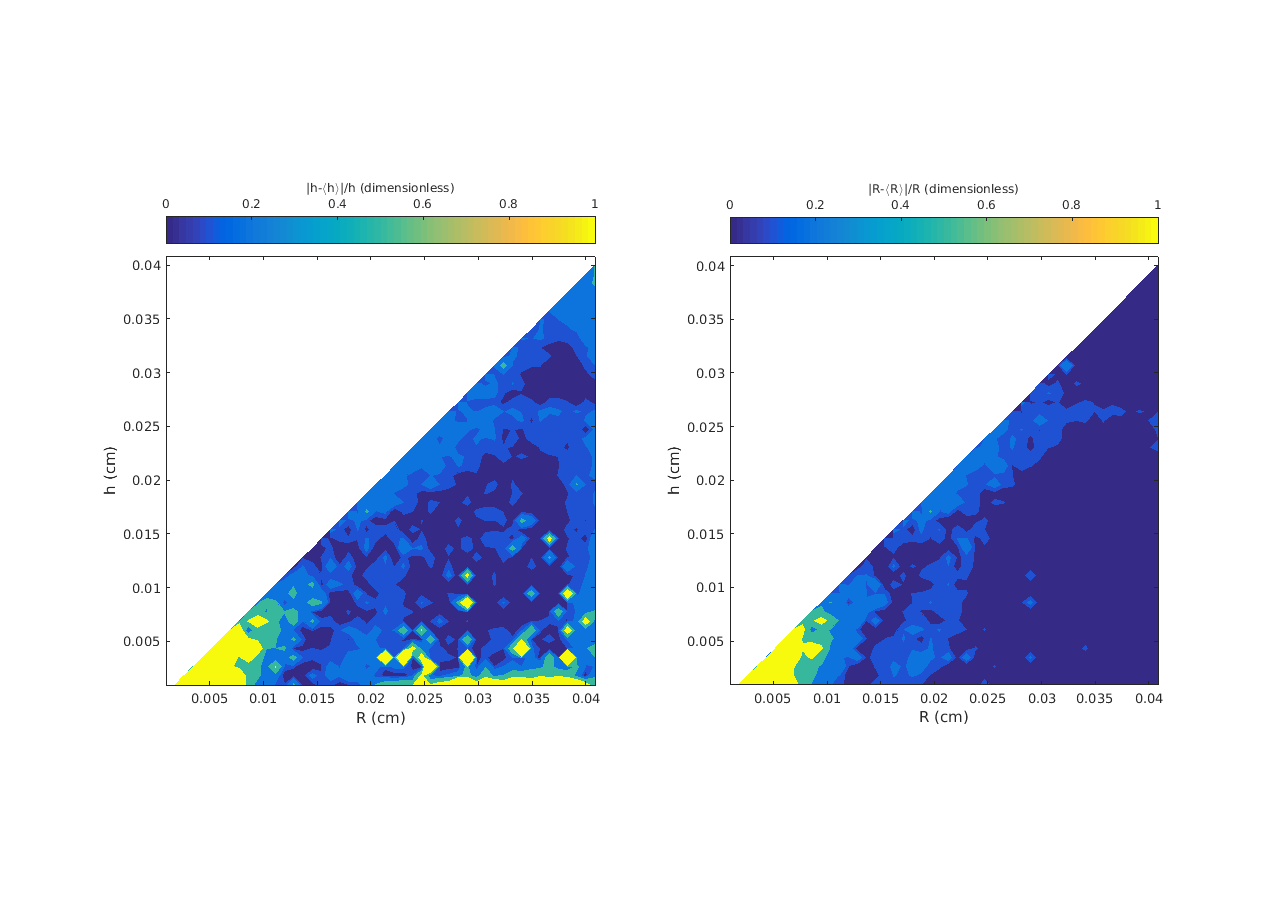
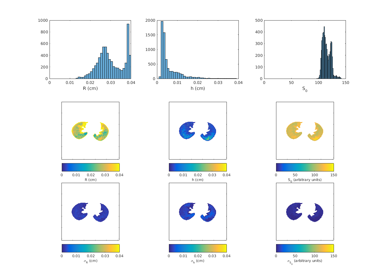
The phantom studies show that the model and MCMC fits are robust for dimensions in the expected physiological range of $$$R = 200-400$$$ μm and $$$h = 100-200$$$ μm. Estimated errors on the order of 50% for $$$R > 200$$$ μm and $$$h > 200$$$ μm are shown in Figure 1. Corresponding image results and estimates of uncertainty in the model fit for a typical normal subject are shown in Figure 2.
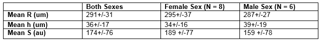
Note that the $$$R$$$ values are consistently larger than their corresponding $$$h$$$ values as expected for the model geometry. A summary of $$$R$$$ and $$$h$$$ values for all subjects appears in Table 3. We compared the $$$h/R$$$ values from female subjects to male subjects with an ANOVA.
Discussion
With the current study population there is no difference in acinar structures in the study subjects. Future work will analyze the larger 40 subject data-set and allow for comparisons between sex, diagnosis of asthma, and pulmonary function tests. Another goal is to investigate regional relationships. In the histogram of $$$R$$$ in Figure 2, there is a buildup of fits in high bins, corresponding to values in the range from 350-400 μm. From the maps in Figure 2, large values of $$$R$$$ appear at the edges of the lung. This location would be consistent with air trapping, but may also be due to partial volume artifact instability in the model fits in the 350-400 μm region. Future work can independently validate these measures using other DWI models and regional measures of CT density.Conclusions
The morphometric technique using DWI has the potential for measuring acinar airway dimensions and alveolar depth at scales appropriate to study pediatric asthma, which may provide insights into acinar dimensions and their regional heterogeneity in asthma.Acknowledgements
AM was supported by NIH/NHLBI P01 HL070831 and and by the National Cancer Institute of the National Institutes of Health under Award Number T32CA009206. The content is solely the responsibility of the authors and does not necessarily represent the official views of the National Institutes of Health. Other authors and activities were supported by NHLBI P01 HL070831 (COAST); The Hartwell Foundation; The Department of Medical Physics and School of Medicine and Public Health, UW-Madison; NIH S10 OD016394 (Pulmonary Imaging Center) .References
1. Paiva M. Gaseous diffusion in an alveolar duct simulated by a digital computer. Comput Biomed Res. 1974 Dec;7(6):533-43.
2. O'Halloran RL, Holmes JH et al. The effects of SNR on ADC measurements in diffusion-weighted hyperpolarized He-3 MRI .J Magn Reson. 2007 Mar;185(1):42-9.
3. Wang W, Nguyen NM, et al. Imaging lung microstructure in mice with hyperpolarized 3He diffusion MRI. Magn Reson Med. 2011 Mar;65(3):620-6.
4. Parra-Robles J, Wild JM. The influence of lung airways branching structure and diffusion time on measurements and models of short-range 3He gas MR diffusion. J Magn Reson. 2012 Dec;225:102-13.
5. Kruger SJ, Nagle SK et al. Functional imaging of the lungs with gas agents. J Magn Reson Imaging. 2016 Feb;43(2):295-315.
6. Hajari AJ, Yablonskiy DA, et al. Morphometric changes in the human pulmonary acinus during inflation.J Appl Physiol (1985). 2012 Mar;112(6):937-43.
7. Quirk JD, Sukstanskii AL, et al. Experimental evidence of age-related adaptive changes in human acinar airways.J Appl Physiol (1985). 2016 Jan 15;120(2):159-65.
8. Cadman RV1, Lemanske RF Jr, et al. Pulmonary 3He magnetic resonance imaging of childhood asthma. J Allergy Clin Immunol. 2013 Feb;131(2):369-76.e1-5
9. Sukstanskii AL, Yablonskiy DA. In vivo lung morphometry with hyperpolarized 3He diffusion MRI: theoretical background. J Magn Reson. 2008 Feb;190(2):200-10.
10. Yablonskiy DA, Sukstanskii AL, et al. Quantification of lung microstructure with hyperpolarized 3He diffusion MRI. J Appl Physiol. 2009 Oct;107(4):1258-65.
11. Sukstanskii AL1, Bretthorst GL, et al. How accurately can the parameters from a model of anisotropic 3He gas diffusion in lung acinar airways be estimated? Bayesian view. J Magn Reson. 2007 Jan;184(1):62-71.Figures