3019
A Least Squares Approach for Relative Pressure Measurement from 4D flow PC-MRI1Biomedical Engineering, School of Advanced Technologies in Medicine, Isfahan University of Medical Science, Isfahan, Iran (Islamic Republic of), 2Electrical and Computer Engineering, University of Louisville, Louisville, KY, United States
Synopsis
Noninvasive determination of relative
Introduction
Noninvasive and accurate measurement of pressure drop across arterial and valvular stenosis is important as pressure drop a significant physiological indicator which may be used to assess the severity of the disease. Assuming blood to be an incompressible laminar Newtonian fluid, the blood flow velocity obtained from 3D PC-MRI can be used as the input to the Navier-Stokes equation to determine the pressure gradient field in a vessel. But due to noise, the integration of resulting pressure gradient will not be path independent.
Pressure Poisson Equation (PPE)1 and Harmonic –Based Orthogonal Projection using FFT2 were previously introduced for solving this problem. In this abstract, we propose a fast matrix-based method for Least-Square (LS) reconstruction of the relative blood pressure.
Method
For the fluid with constant viscosity $$$(\mu)$$$, the Navier-Stokes equation for steady flow can be expressed as: $$$\widehat{\triangledown P}=-\rho(u.\triangledown)u+\mu \triangledown^{2}u+\rho f$$$ where $$$\widehat{\triangledown P}=(\widehat{P_{x}},\widehat{P_{y}},\widehat{P_{z}})$$$ is the pressure gradient field, $$$u(x,y,z)$$$ is the measured 3-dimensional velocity, $$$\rho$$$ is the fluid density and $$$f$$$ is the body force. To reduce the distance between the gradients of reconstructed pressure $$$\widetilde{P}$$$ and measured pressure $$$\widehat{P}$$$, the error function: $$$\epsilon=\sum_{\Omega_{f}}^{}|\widehat{\triangledown P}-\widetilde{\triangledown P}|^{2}$$$ should be minimized over the flow domain $$$\Omega_{f}$$$. Supposing $$$G$$$ is the discrete differentiation matrix with proper dimensions, the partial derivatives of the $$$\widetilde{P}$$$ can be written as: $$$\frac{\partial \widetilde{P}}{\partial I}=G_{I}\widetilde{P}$$$ with $$$I=x,y,z$$$. Considering this matrix-based approach, the error function can be rewritten as sum of squared differences:$$\epsilon=\sum_{\Omega_{f}}^{}|\widehat{P_{x}}-G_{x}\widetilde{P}|^{2}+|\widehat{P_{y}}-G_{y}\widetilde{P}|^{2}+|\widehat{P_{z}}-G_{z}\widetilde{P}|^{2}$$ Note that, $$$G_{x}$$$, $$$G_{y}$$$ and $$$G_{z}$$$ can be chosen as any finite difference approximation scheme including second order or higher central/eccentric difference scheme. Minimizing $$$\epsilon$$$ with respect to unknown variable $$$\widetilde{P}$$$ leads to following formula as derived in [3]:$$(I_{z}\otimes I_{y}\otimes G_x^TG_{x}+I_{z}\otimes G_y^TG_{y}\otimes I_{x}+G_z^TG_{z}\otimes I_{y}\otimes I_{x} )\widetilde{P}=(I_{z}\otimes I_{y}\otimes G_x^T\widehat{P_{x}}+I_{z}\otimes G_y^T\widehat{P_{y}}\otimes I_{x}+G_z^T\widehat{P_{z}}\otimes I_{y}\otimes I_{x})$$ Where I indicates identity matrix and $$$\otimes$$$ denotes Kronecker tensor product. Clearly, the right hand side of this equation maybe directly computed from measured pressure gradients. But the main issue for constructing the pressure, is the inverse calculation of the left side which multiplies $$$\widetilde{P}$$$ which could be done efficiently by substituting the $$$G^{T}G$$$ matrix with its Eigen decomposition form.
Blood pressure could be estimated by this approach non-iteratively provided that valid measurement flow exists on entire rectangular domains of the image. However, in the case of PC-MRI data, vessel lumen does not cover whole image domain and there is no flow information outside of the vessel. To handle this issue, an iterative LS scheme, proposed by Wang 3 , was applied. To do this, all pressure gradient values out of $$$\Omega_{f}$$$ initialize by zeros and after employing LS scheme to obtain pressure field, in the next step, their values are updated by the gradient of the recently reconstructed pressure field. This procedure is continued until a specific termination criterion is satisfied.
Materials
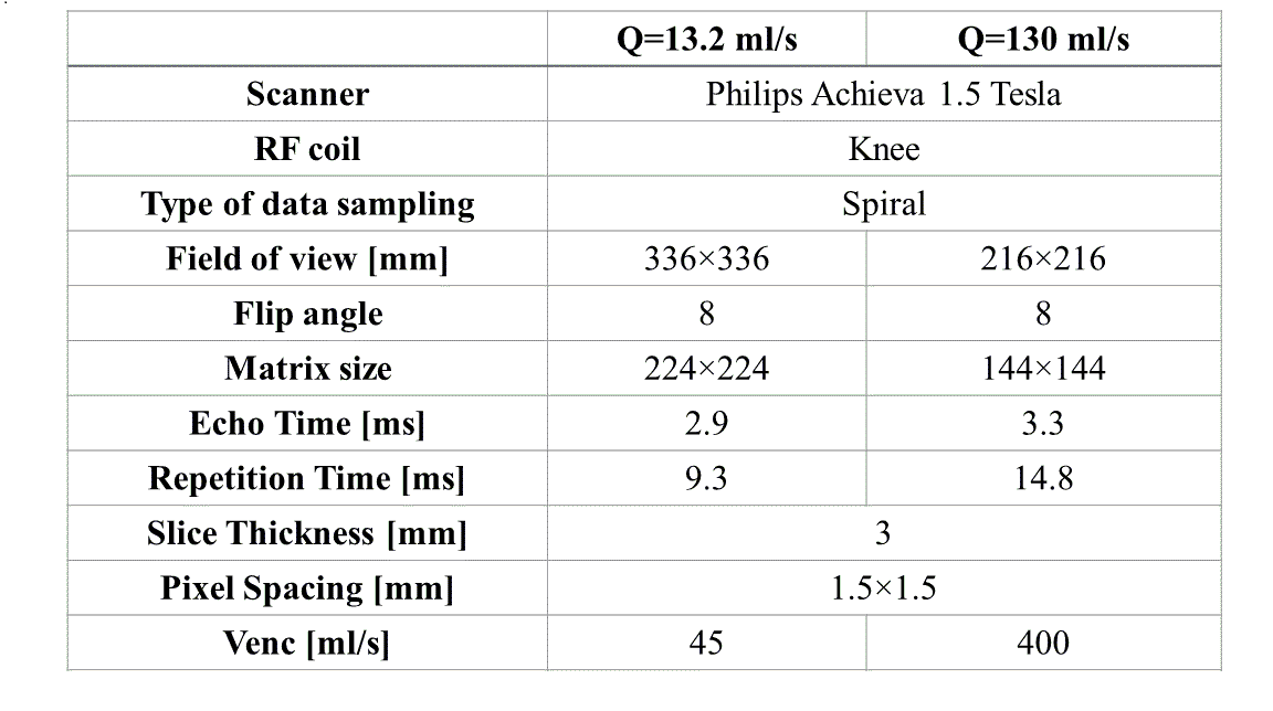
Experiments were applied on two types of data, Computational Fluid Dynamic (CFD) and MRI flow phantom. To simulate a stenosis valve, in the case of CFD, a 3D geometrical cylinder model with 90% area stenosis was created and steady Navier-Stokes equations were numerically solved over 8 million tetrahedral finite element mesh at flow rate=13.2 ml/s. For in-vitro studies, a closed loop flow system phantom with a 75% and 87% stenosis was run at 13.2 ml/s and 130 ml/s flow rates respectively. The imaging parameters are shown in Table 1.Results
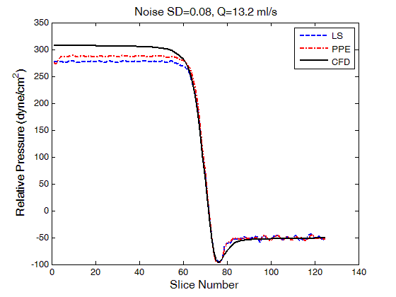
To evaluate the effect of the noise, LS and PPE methods were fed by noise-corrupted CFD velocity fields with zero mean additive Gaussian noise. Figure 1 depicts the comparison between true pressure calculated directly by CFD and those derived from LS and PPE solutions when using noise-corrupted CFD velocity data. As can be seen, there is a good agreement between two approaches and CFD pressures.
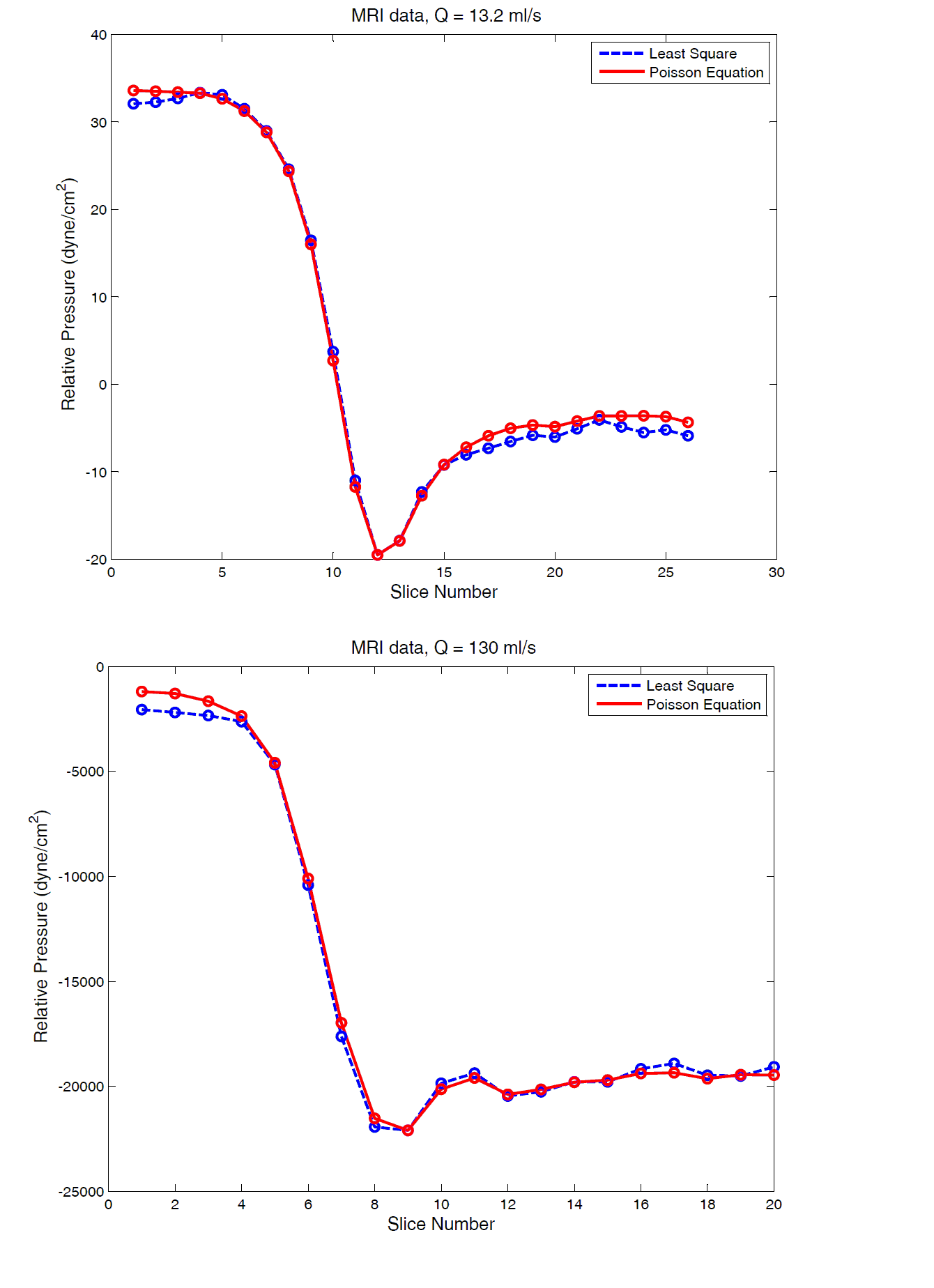
The results of LS and PPE methods on MRI data at 13.2 ml/s and 130 ml/s flow rates are shown in figure 2. The new method follows PPE quite closely. The computational time for the LS approach is 8.8 seconds which is to be compared to 123 seconds for PPE scheme on a machine with a dual-core 3GHz processor and 8GB RAM.
Conclusion
This paper introduced a 3D matrix-based least square solution for measuring relative transstenotic pressure drop from PC-MRI. The results of both CFD simulation and phantom MRI data demonstrated the acceptable performance of the LS algorithm. Further work remains to show the utility of the method in deriving pressures from pulsatile and in-vivo data.Acknowledgements
No acknowledgement found.References
1. A.N.Moghaddam, et al., Magn Reson in Med (2004), vol. 52, pp. 300-309.
2. MJ.Negahdar, et al, Proc Intl Soc Mag Reson Med. 21 (2013)
3. Wang, C.Y, et al. Exp Fluids (2017), pp. 58-84. DOI: s00348-017-2368-0
Figures