Synopsis

In Dynamic Contrast-Enhanced (DCE) MRI, inaccurate estimation of the arterial input function (AIF) is still a major cause of the low reliability of kinetic parameter estimates. We propose a new method of AIF estimation. It combines AIF measured from the blood-pool signal and multichannel blind deconvolution. The weights of the measured AIF are based on its analytically derived uncertainty and a model relating signal intensity and gadolinium concentration.

The method has been evaluated on simulated myocardial perfusion data, mimicking real noise and kinetic parameter distributions. The hybrid method gave better results compared to the blood-pool or blind-deconvolution approaches alone.

Introduction

Dynamic Contrast-Enhanced (DCE) MRI is an important method for assessment of microvascular tissue parameters. However, inaccurate estimation of the arterial input function (AIF) is still a major cause of the low reliability of kinetic parameter estimates. The AIF is commonly determined from the measured blood-pool signal, which can be inaccurate due to saturation, T2*, flow and partial-volume effects. Alternatively, AIF can be obtained with a dual-bolus acquisition¹ (increasing scan time), using population-based AIF² (ignoring the differences in patients' vascular-tree status and in acquisition methods) or reference-tissue methods³ (assuming known perfusion parameters in a reference tissue). Blind deconvolution^4,5 is an alternative approach that avoids many above-mentioned problems. With blind deconvolution, the AIF is estimated from several tissue concentration curves that have all “seen” the same AIF. To provide a unique solution, blind deconvolution requires sufficient variability in the input tissue curves. This can be a challenge, especially in regions of healthy myocardial tissue.

Here we combine AIF estimation from the blood-pool signal and multichannel blind deconvolution to achieve better reliability. This work is an extension of an approach⁶ where a part of the measured AIF under a heuristically set threshold was combined with blind deconvolution. We propose a formalized method to set the weights of the measured AIF based on its analytically derived uncertainty and a model relating signal intensity and gadolinium concentration.

Methods

The parameterized⁵ AIF (vector $$$C_a$$$) is estimated by minimizing

$$ \lambda \sum_{n=1}^N ||C_{n}-H_n C_a ||_2^2 + (1-\lambda) ||w [f(C_a) - S_a] ||_2^2$$

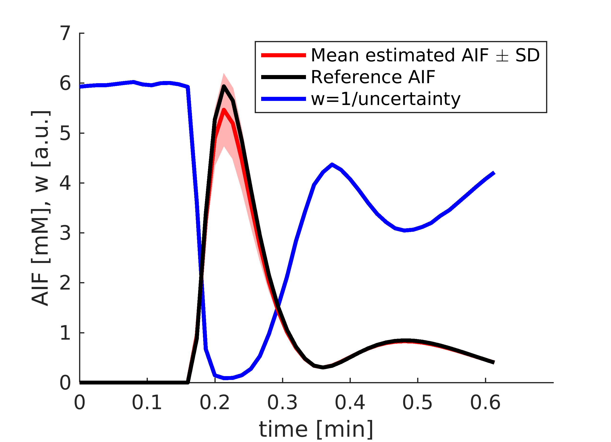
The first (blind-deconvolution) term approximates each $$$n$$$-th measured tissue concentration signal (vector $$$C_n$$$) by convolution of its tissue residual function (matrix $$$H_n$$$) and the AIF. The matrix $$$H_n$$$ represents the extended Tofts model⁷ and the convolution is expressed as matrix multiplication. The second (conversion) term approximates the measured blood-pool signal, vector $$$S_a$$$, by the acquisition model $$$f (C_a)$$$. The weights of the two terms are controlled by $$$\lambda$$$ (here set experimentally). The weight vector $$$w$$$ is the reciprocal of the uncertainty of $$$C_a$$$ given $$$S_a$$$ and an acquisition model. The uncertainty is derived analytically for saturation-recovery radial-sampling FLASH, including the effect of excitation pulses and T2* (the derivation is similar to that done for steady-state GRE⁸). This formulation assigns low weight to high gadolinium concentration (AIF peak) reflecting the uncertainty created by the saturation effect (Fig.1).

The method has been evaluated on simulated cardiac DCE-MRI data: 500 synthetic concentration curves were generated mimicking myocardial single-voxel signals of one slice with realistic noise and distribution of perfusion parameters⁶. These signals were then k-means clustered into $$$N$$$=10 clusters yielding the $$$C_n$$$ signals⁴. This was repeated 5x for different noise realizations. The reference AIFs were derived from a real low-dose (0.004 mmol/kg) DCE-MRI acquisition by scaling to the simulated dose levels. The signals $$$S_a$$$ were generated from the reference AIFs using the acquisition model $$$f$$$, including the T2* effect (MultiHance: r2*=17.5L/mmol/s).

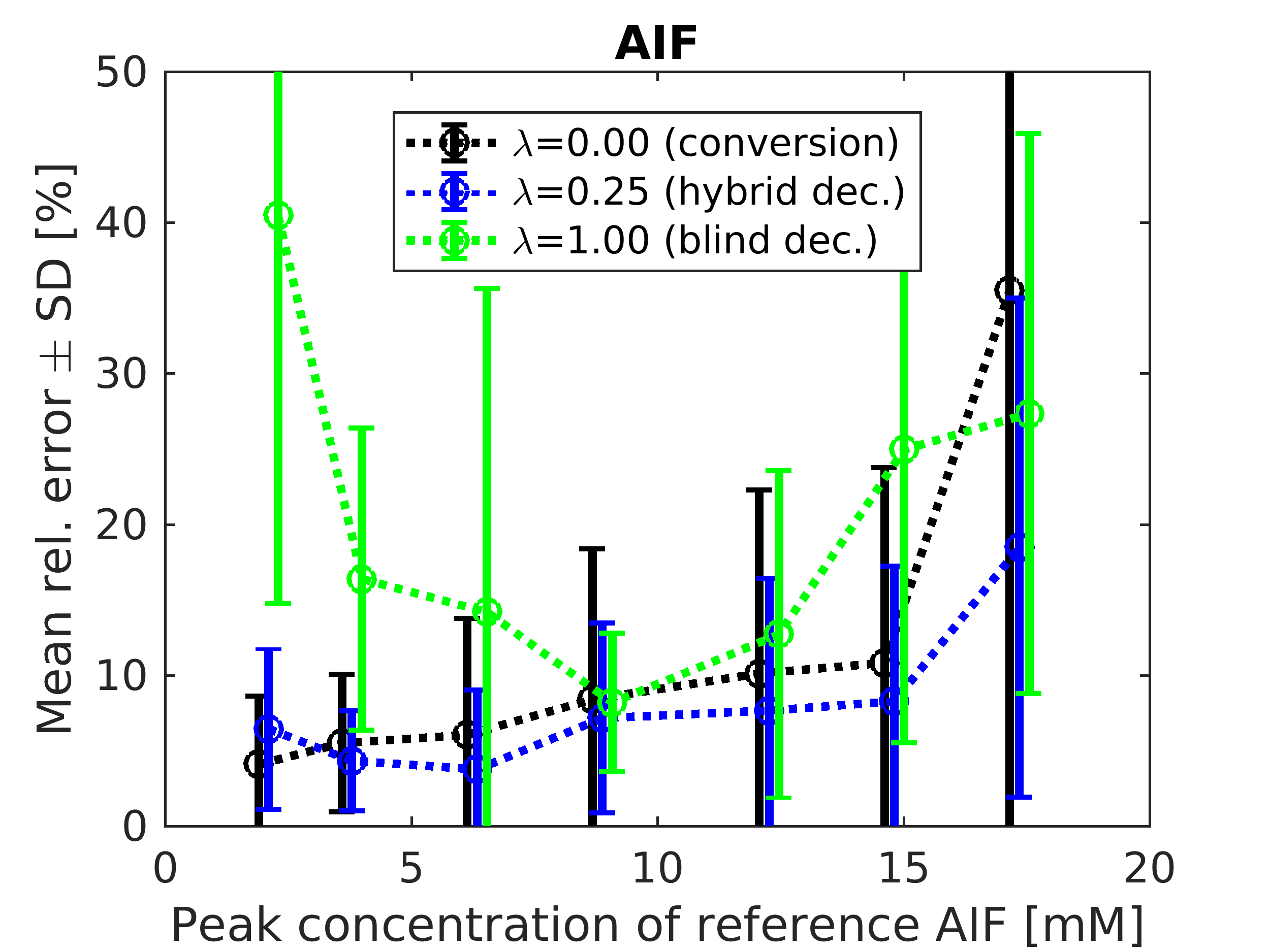
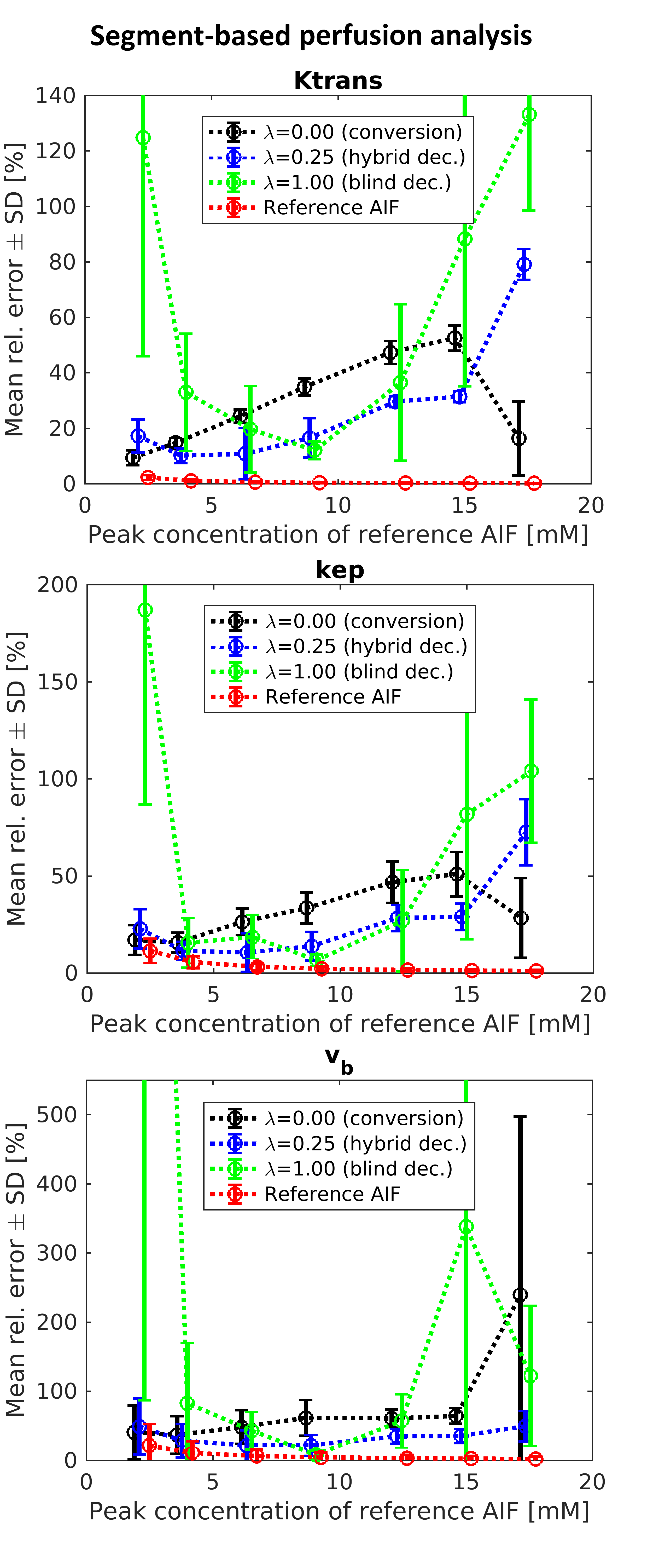
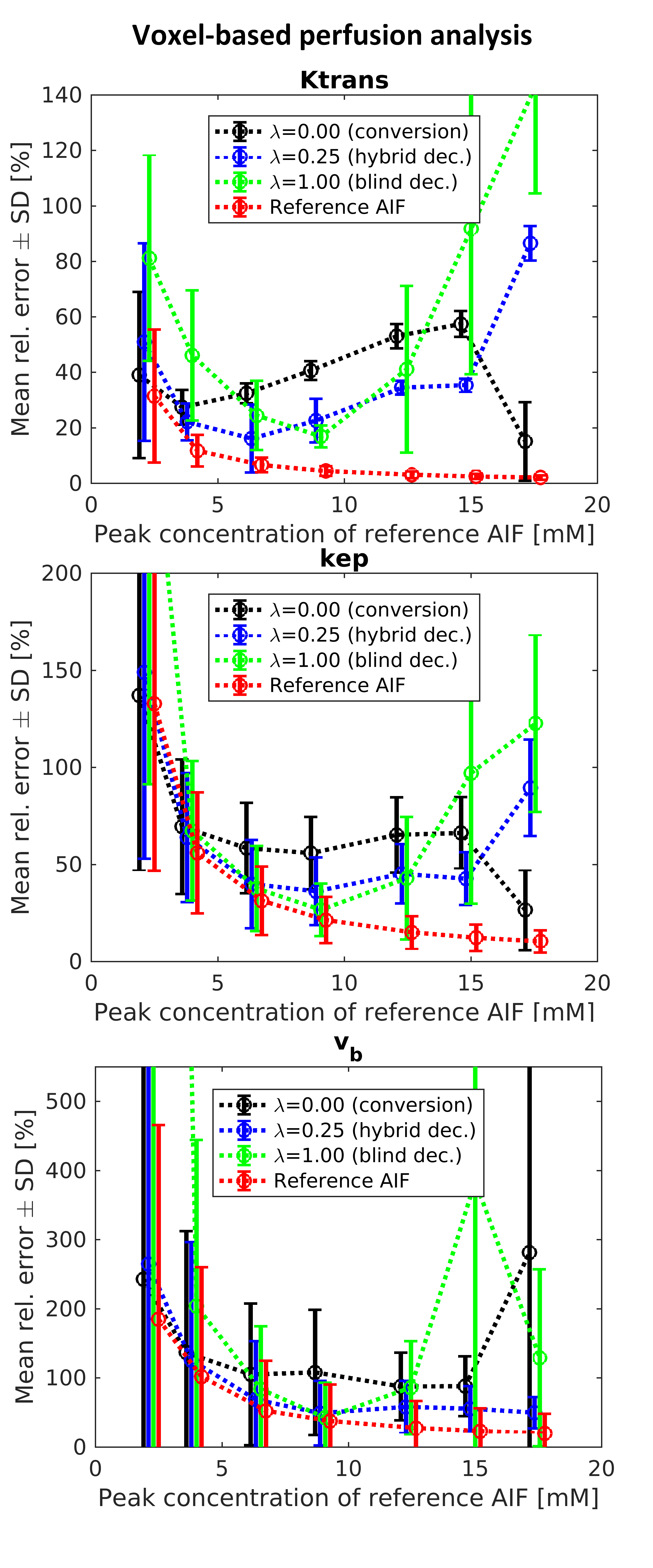
The accuracy of AIF estimation has been evaluated using its relative error (Fig.2) and relative errors of the kinetic parameters estimated in the subsequent non-blind deconvolution with the estimated AIFs (Figs.3-4).

Results

Using only the signal-to-concentration conversion term (λ=0), the accuracy of AIF estimation and the corresponding kinetic-parameter estimates improved with lower injection dose (Figs.2-4). For the highest dose, the accuracy of $$$K^{trans}$$$ and $$$k_{ep}$$$ seemingly improved, probably as a result of outlying $$$v_b$$$ estimates (Figs.3-4). Using only the blind-deconvolution term (λ=1), AIF estimation performed poorly for too low (due to poor SNR) and too high (due to inaccurate initial AIF estimation, here derived from $$$S_a$$$) injection doses (Figs.2-4). The hybrid AIF estimation (0<λ<1) was the most accurate, except for the lowest injection dose where the conversion method was better.

Discussion

As expected, the conversion term alone leads to precise AIFs in low-concentration range but introduces errors for higher concentrations where the T2* effect (included here when simulating the signal from the true AIF but not when estimating the AIF) violates the acquisition model $$$f(C_a)$$$ where the T2* effect is not included. T2* could be estimated as well but has additional challenges⁹. Combining the signal-to-concentration conversion weighted by uncertainty with blind deconvolution gives more accurate and more robust AIF estimation for a range of gadolinium dose levels. This hybrid approach also solves the problem of undefined scale and shift of blind-deconvolution AIF estimation.

Conclusion

Acknowledgements

This work was supported by grants from the Czech Science Foundation (grant no. 16-13830S), by the Ministry of Education, Youth, and Sports of the Czech Republic (project No. LO1212) and NIH R01HL135328.

References

1. Kostler H, Ritter C, Lipp M, et al. Prebolus quantitative MR heart perfusion imaging. Magn Reson Med. 2004;52(2):296–299.

2. Parker GJM, Roberts C, Macdonald A, et al. Experimentally-derived functional form for a population-averaged high-temporal-resolution arterial input function for dynamic contrast-enhanced MRI. Magn Reson Med. 2006;56(5):993–1000.

3. Yankeelov TE, Luci JJ, Lepage M, et al. Quantitative pharmacokinetic analysis of DCE-MRI data without an arterial input function: A reference region model. J Magn Reson Imaging. 2005;23(4):519–529.

4. Fluckiger JU, Schabel MC, DiBella EV. Model-based blind estimation of kinetic parameters in dynamic contrast enhanced (DCE)-MRI. Magn Reson Med. 2009;62(6):1477–1486.

5. Schabel MC, Fluckiger JU, DiBella EVR. A model-constrained Monte Carlo method for blind arterial input function estimation in dynamic ontrast-enhanced MRI: I. Simulations. Phys Med Biol. 2010;55(16):4783–4806.

6. Fluckiger JU, Schabel MC, DiBella EVR. Constrained estimation of the arterial input function for myocardial perfusion cardiovascular magnetic resonance. Magn Reson Med. 2011;66(2):419–427.

7. Tofts PS, Brix G, Buckley DL, et al. Estimating kinetic parameters from dynamic contrast-enhanced T1-weighted MRI of a diffusible tracer: Standardized quantities and symbols. J Magn Reson Imaging. 1999;10(3):223–232.

8. Schabel MC, Parker DL. Uncertainty and bias in contrast concentration measurements using spoiled gradient echo pulse sequences. Phys Med Biol. 2008;53(9):2345–2373.

9. van Osch MJ, Vonken EJ, Viergever MA, et al. Measuring the arterial input function with gradient echo sequences. Magn Reson Med. 2003;49(6):1067–1076.