2954
Left Ventricle 2D and 3D Strain Phantoms Generation Using a Python Finite Element-based Library1Biomedical Imaging Center, Pontificia Universidad Católica de Chile, Santiago, Chile, 2Electrical Engineering Department, Pontificia Universidad Católica de Chile, Santiago, Chile, 3Radiology Department, Pontificia Universidad Católica de Chile, Santiago, Chile, 4Institute for Biological and Medical Engineering, School of Engineering, Medicine and Biological Sciences, Pontificia Universidad Católica de Chile, Santiago, Chile
Synopsis
The strain in the left ventricle is a well-known biomarker for cardiac diseases. Nowadays, several acquisition techniques have been developed to improve the diagnose of this kind of conditions. Usually, strain biomarkers are obtained by mean of image post-processing techniques using different deformation metrics. In this work we present a numerical framework for the generation of left-ventricle strain phantoms using three different acquisition sequences in order to provide a broad database of patients and volunteers with different types of diseases. Our library provides a robust image generation tool to compare and develop new post-processing methods for quantifying strain phantoms
Introduction
The strain in the left ventricle is a well-known biomarker for the assessment of different cardiac diseases. Nowadays, several acquisition techniques have been developed to improve the estimation of strain parameters. Two of the most important approaches are Tagging1 and Displacement Encoding with Stimulated Echoes2 (DENSE), the actual and the next gold standard for strain estimation3. There are also some reports using tissue velocity mapping4 (TVM), which comes from phase contrast MR5 measurements.
Strain parameters are obtained from different deformation metrics using post-processed images. In the case of tagging and DENSE, the metric is usually the strain tensor, whereas strain rate4 is used in TVM data. One way to analyse the results of these methods is the use of numerical phantoms. However, to the best of our knowledge there is no numerical phantom available that provides data for a direct comparison between Tagging, DENSE and TVM techniques.In this work, we propose an numerical phantom which in combination with the Bloch equation can provide data for the analysis of Tagging, DENSE and TVM simultaneously. Furthermore, the phantom can simulate data from volunteers or patients.Methods
The direct quantification of the strain in the left ventricle considers the displacement field $$$\vec{\boldsymbol{u}}$$$, acquired using tagging or DENSE techniques. Alternatively, 2D or 3D velocity fields $$$\vec{\boldsymbol{v}}$$$ from TVM can also provide qualitative strain measures4 from strain rate calculations.
The library is composed by multiple functions (written in Python programming language) that can be divided in three modules: (I) the generation of displacement fields, (II) post-processing and interpolation of data to images and (III) reading and writing. The first module is performed by solving the hyperelastic equations using an open source finite elements library called FEniCS6 or with the generation of analytical phantoms7. The second module uses the numpy8 and FEniCS libraries to mimic the three previously described sequences. The image construction is performed knowing the expression of the magnetization for the three acquisition sequences. The tagging images are generated using the SPAMM9 sequence, from which the tag-lines are distributed spatially according to
$$ M_{xy} = M_0 e^{-t/T_1}(\cos^2\alpha + \sin^2\alpha\cos^2(k_e x_i) - 1) + M_0 $$
where $$$M_0$$$ is thermal equilibrium magnetization, $$$\alpha$$$ the flip angle, $$$k_e$$$ the encoding frequency and $$$x_i$$$ the position in the direction $$$i$$$. In the case of DENSE and PC-MR the relation between the phase $$$\Delta\phi$$$ and the displacements and velocities (respectively) has been deeply studied5,10 and took the form
$$ \Delta\phi_{x_i} = k_e u_i, \qquad \Delta\phi_{x_i} = \frac{v_i \pi}{\text{venc}} $$
where the encoding frequency $$$k_e$$$ (also for SPAMM) is given by
$$ k_e=\gamma\int_{\Delta T} G_{x_i}(\tau)d\tau $$
and where $$$\Delta T$$$ and $$$G_{x_i}$$$ are the encoding time and gradient, respectively.
The last module consist of reading and writing functions that can export the phantom simulations into DICOM images and VTK files (displacement and velocity fields).
We used this library to simulate numerical 2D and 3D dynamic phantoms that provide a FE mesh with a displacement field. The 2D phantoms consist of two concentric circles that moves with a prescribed displacement as explained in Gilliam et al8. The 3D phantom was obtained by solving the hyperelasticity equations over an idealized geometry of the left-ventricle11. The 2D and 3D ventricle geometries are then deformed using the obtained field displacements. This deformed geometry is finally used to build Tagging, DENSE and TVM images with the equations described above.
Results
Figures 1 and 2 shows the FE results obtained with our library for 2D and 3D phantoms. The resulting 2D and 3D images are appreciated in Figures 3 and 4. In both figures, we show the resulting images for one simulated volunteer and one patient. For both phantoms the displacements and velocities are between physiological ranges.
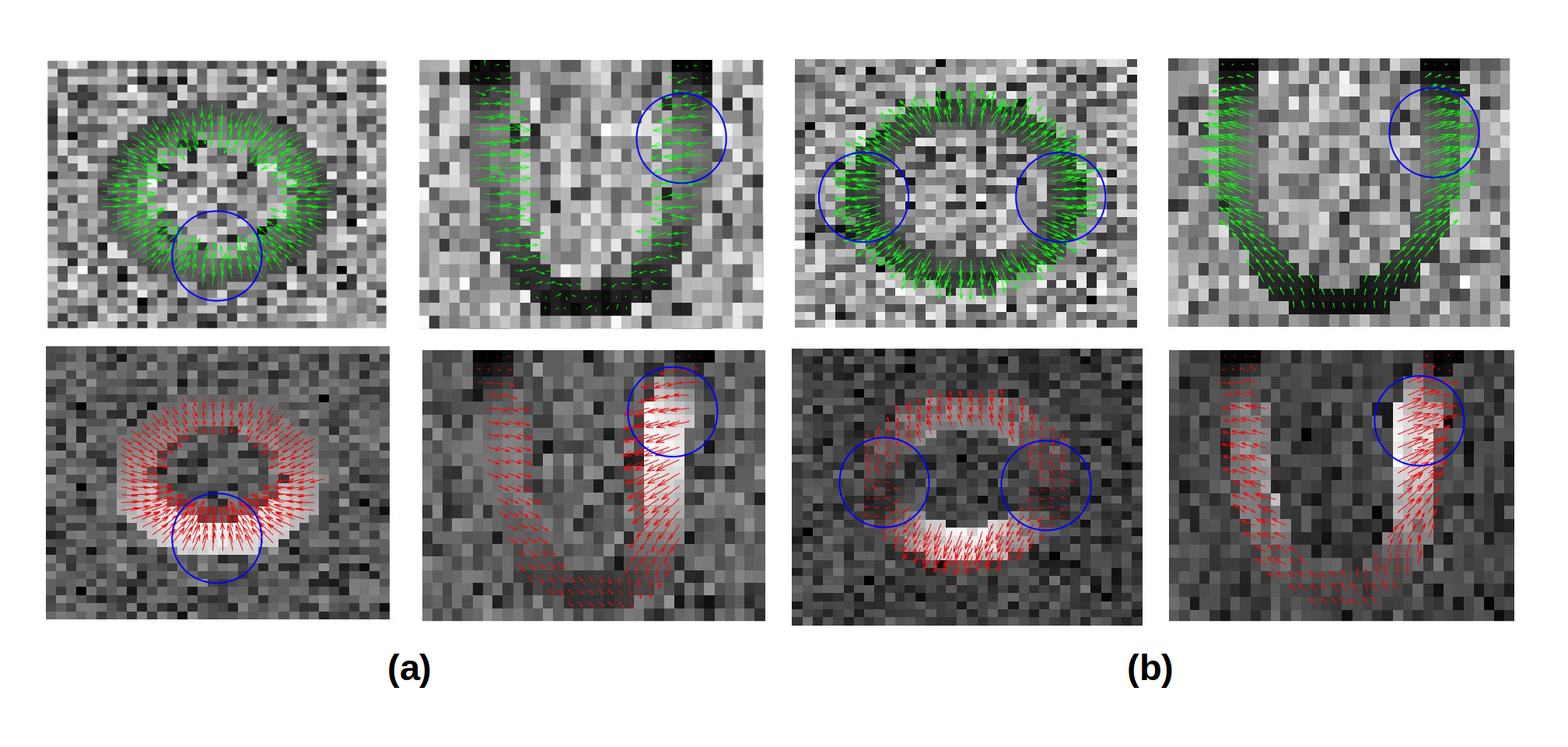
In Figure 3 we can appreciate differences in the displacements fields, i.e, in how the ventricle is being deformed, whereas in Figure 4 places with higher and different displacements and velocities are indicated in blue circles. For the last case, the phantom simulating a patient condition was obtained changing the stiffness of the free wall at the basal level.
Discussion and Conclussion
The quantification of the cardiac mechanics from MRI strain evaluations is a very active research field and requires permanent improvements. We presented an efficient FE based library for the generation of numerical phantoms for strain quantification. We can generate a large variety of conditions using the numerical 2D and 3D in-silico phantoms.This Python library is useful for a wide range of research and academic purposes. Inspired by the necessity of continuous development and comparison of novel techniques for the post-processing, this code has DENSE, SPAMM, and TVM techniques implemented, but is open to other methods as well.Acknowledgements
We thank to CONICYT-PIA-Anillo ACT1416, CONICYT FONDEF/I Concurso IDeA en dos etapas ID15/10284 and FONDECYT #1141036, FONDECYT Postdoctorado 2017 #3170737 and National PhD scholarship N3455/2017 grants.
References
- Axel L, Montillo A, Kim D. Tagged magnetic resonance imaging of the heart: a survey. Med Image Anal. 2005 Aug;9(4):376-93.
- Kim D, Gilson WD, Kramer CM, Epstein F. Myocardial Tissue Tracking with Two-dimensional Cine Displacement-encoded MR Imaging: Development and Initial Evaluation. Radiology. 2004 230(3):862-871.
- Auger D. Cardiac Mechanics. Proc. Intl. Soc. Mag. Reson. Med. 25 (2017).
- Nayak KS. Cardiovascular magnetic resonance phase contrast imaging. J Cardiovasc Magn Reson. 2015 Aug 9;17:71. doi: 10.1186/s12968-015-0172-7.
- Pelc
NJ,
Bernstein
MA,
Shimakawa
A,
Glover
GH.
Encoding strategies for three-direction phase-contrast MR imaging of
flow.
J
Magn Reson Imaging. 1991 Jul-Aug;1(4):405-13.
- Logg A, Wells GN. DOLFIN: Automated Finite Element Computing. ACM Trans Math Software. 2010 37(2):201-208.
- Gilliam A, Epstein F. Automated Motion Estimation for 2D Cine DENSE MRI. IEEE Trans Med Imaging. 2012 Sep; 31(9): 1669–1681.
- Stéfan van der Walt, S. Chris Colbert and Gaël Varoquaux. The NumPy Array: A Structure for Efficient Numerical Computation. Computing in Science & Engineering. 201113:22-30.
- Axel L, Dougherty L. MR imaging of motion with spatial modulation of magnetization. Radiology. 1989 Jun;171(3):841-5.
- Spottiswoode BS, Zhong X, Hess AT, Kramer CM, Meintjes EM, Mayosi BM, Epstein FH. Tracking myocardial motion from cine DENSE images using spatiotemporal phase unwrapping and temporal fitting. IEEE Trans Med Imaging. 2007 Jan;26(1):15-30.
- Land S. et al. Verification of cardiac mechanics software: benchmark problems and solutions for testing active and passive material behaviour. Proc. R. Soc. 2015 A471: 20150641.
Figures
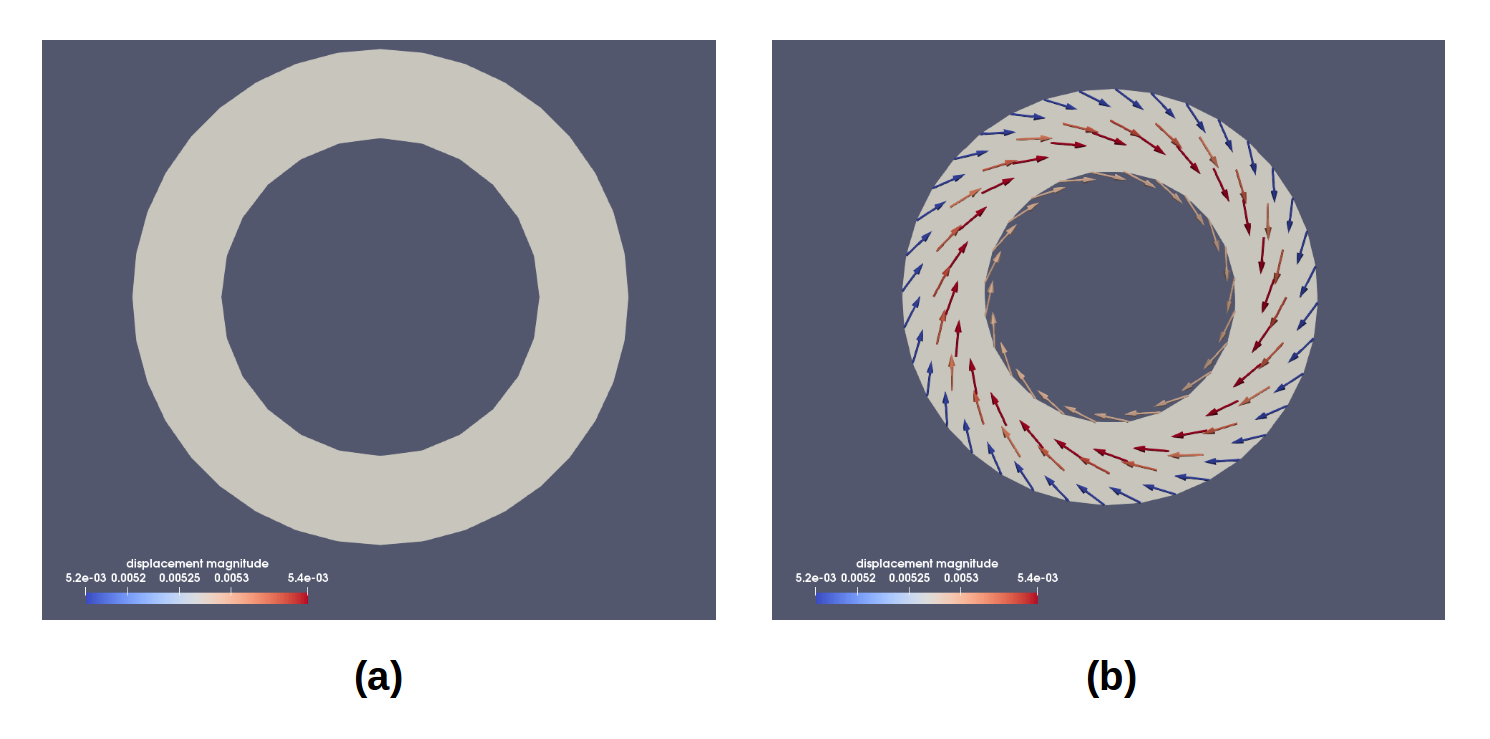
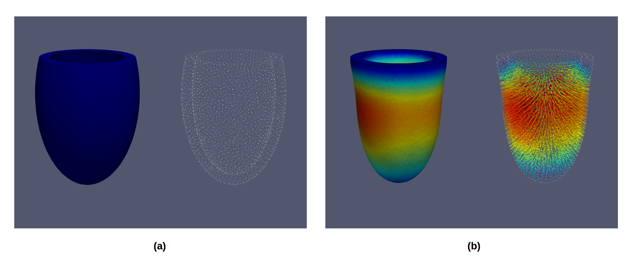
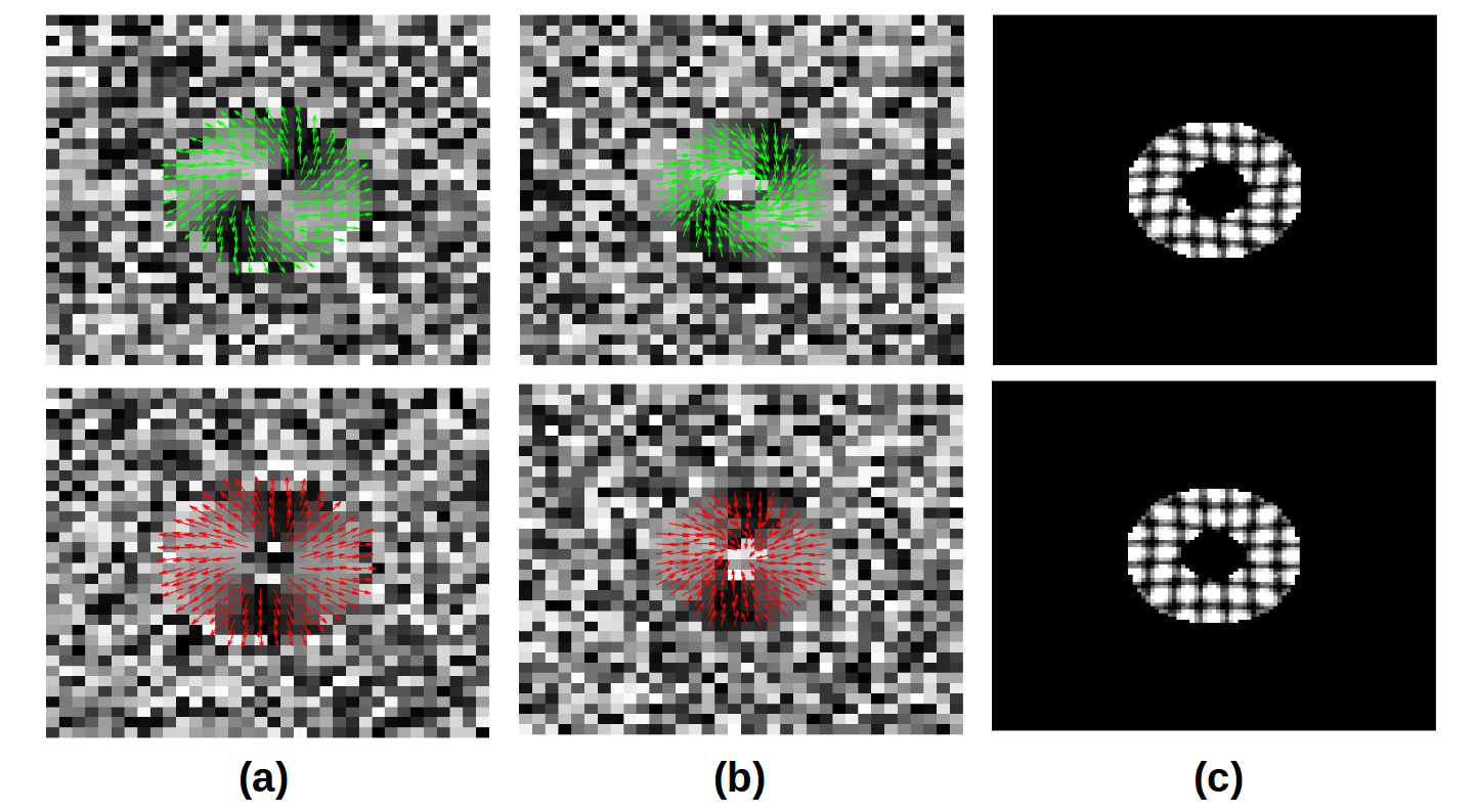
Figure 3: Reconstructed displacements, velocities and tag lines for generated data from (a) DENSE, (b) PC-MR and SPAMM acquisitions for one volunteer (green arrows) and patient (red arrows)