2945
A Validation of MR Flow Velocity Mapping with Automated Phase Offset Correction Using a Gel Flow Phantom Controlled by a Motorized Piston in MR Phase Contrast Cine Flow Measurement1Human Magnetic Resonance Center, Institute of Applied Life Sciences, University of Massachusetts Amherst, Amherst, MA, United States, 2Department of Mechanical and Industrial Engineering, University of Massachusetts Amherst, Amherst, MA, United States
Synopsis
The accuracy of MR flow velocity measurement has been compromised due to a phase offset induced from the eddy current of gradient pulses. An automated correction method of the phase offset had been developed using an image-based algorithm. In order to validate the correction method and the measured velocity accuracy, we developed a flow phantom with a constant flow cross-section and used a servo motor controlled actuator to move the flow phantom accurately. The controlled movement of the new flow phantom allowed us to validate the phase offset correction method and the accuracy of the MR velocity measurement.
Introduction
The accuracy of flow velocity measurement using the MR phase contrast cine flow imaging has been compromised due to phase offset that is induced from the eddy current of the imaging and flow encoding bipolar gradient pulses. The phase offset required manual correction1,2,3 or image-based processing.4,5 However, the existing methods were not applicable to in vivo studies and a new automated correction method was developed using an image-based algorithm.6 This method has been successfully applied to the study of the cerebrospinal fluid (CSF) flow, particularly in spinal cord injury patients.7 However, the correction method and the accuracy of the measured flow velocity have not been validated. The use of liquid flow such as water for the phantom has been difficult due to a laminar flow profile inside the flow tube. Therefore, we developed a flow phantom with a constant flow profile that was moved accurately using a servo motor controlled actuator.Methods
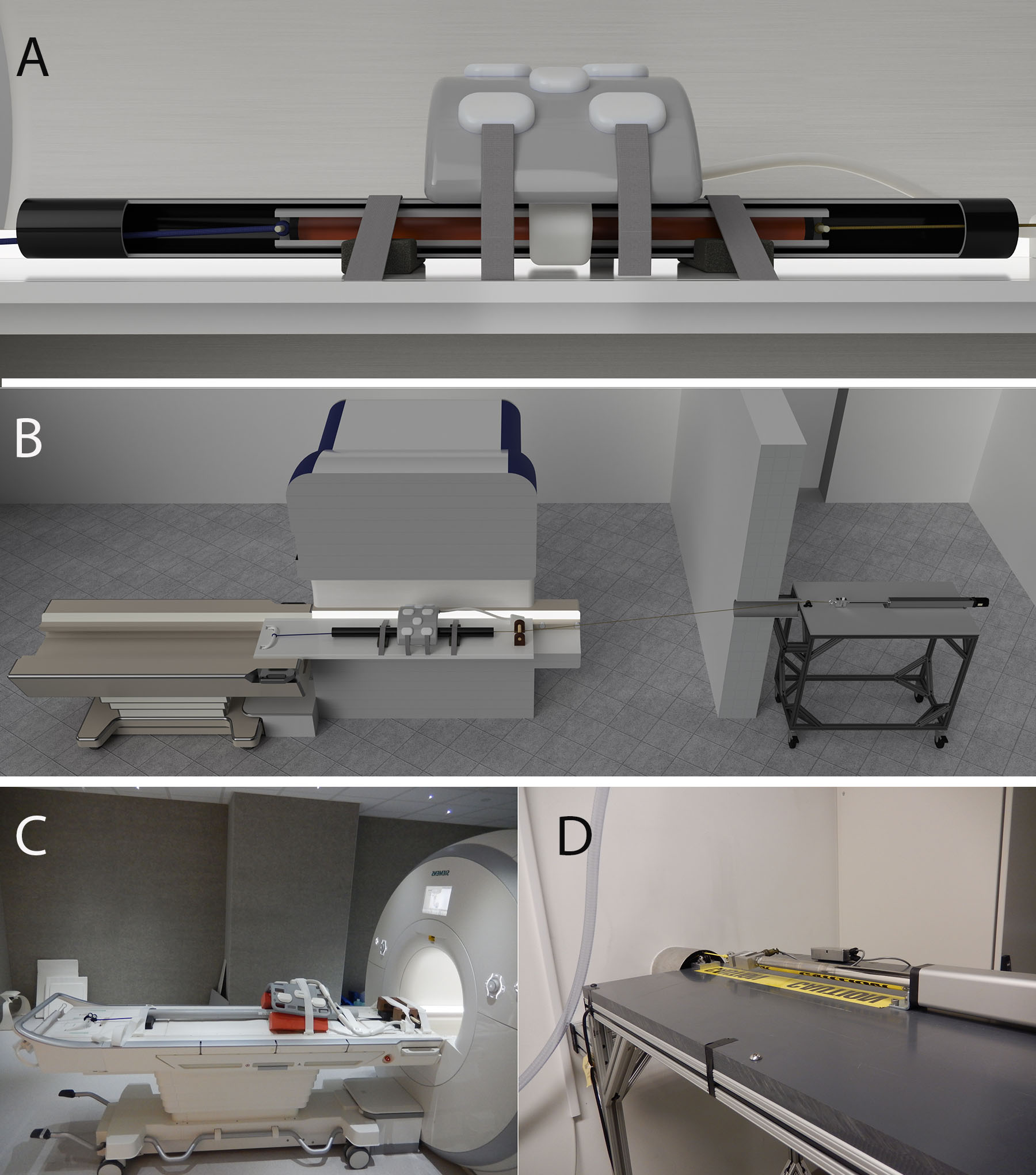
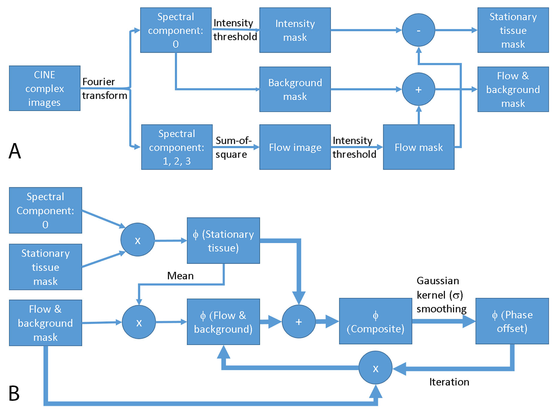
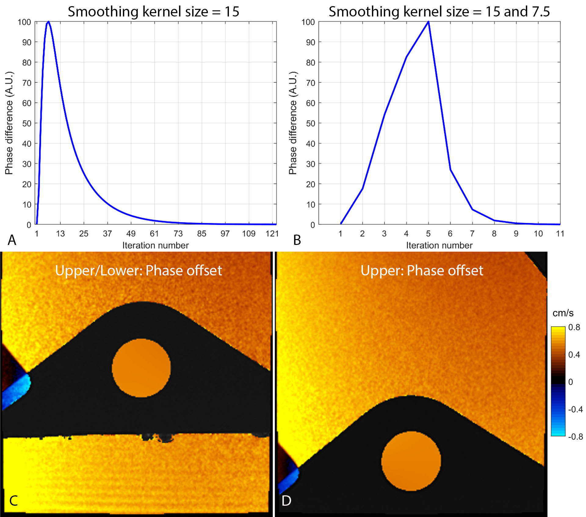
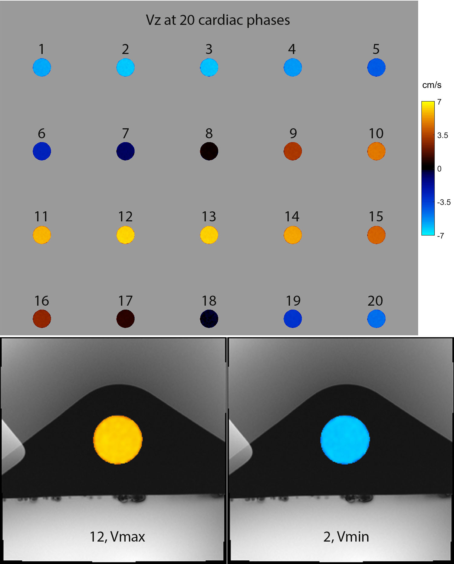
The flow tube was a PVC pipe with an inner diameter of 32mm filled with gel (gelatin) (see Fig. 1). The flow tube was placed in a larger PVC pipe (inner diameter = 51mm). One end of the flow tube was attached to the actuator with a 3mm diameter sheathed Dyneema cable. The other end of the flow tube was pulled in the opposite direction using an elastic cable so that the tube was slid back after being pulled toward the piston. The piston was moved by use of a linear actuator (Thompson PC 40 with a 20-bit encoder) controlled by a microcontroller (Arduino Due). The microcontroller communicated with a supervisory computer to load the motion waveform and motion parameters such as speed and motion range. In addition, the microcontroller reported the motion data to the supervisory computer. The flow PVC tube was configured to be surrounded by stationary phantoms to simulate the spine with the CSF flow. The phantom set was placed on a spine RF coil and covered with a body-array RF coil of a 3T MRI in a similar configuration as the spine flow imaging. A wide rectangular stationary phantom was placed under the flow tube to see the effect of the additional stationary tissue on the phase offset estimation. The piston motion was sinusoidal with a cycle time of 2s for two ranges of ±10mm and ±20mm. The transaxial cine flow images were obtained at two velocity sensitivities of 5 and 10 cm/s in the z direction with a retrospective cardiac gating for 20 cardiac phases using a simulated ECG cycle with the R-R period of 2s. The motor motion and the ECG cycle were periodic with their own clock rate without being synchronized. Other scan parameters were: field-of-view =160 mm, matrix size = 256x256, and slice thickness = 5mm. A Matlab program was developed to segment the flow region and to estimate the phase offset automatically as described in Fig. 2, yielding the cine flow velocity maps over the cardiac cycle.8 The phase offset was estimated iteratively until the absolute difference of the mean phase offset in the flow region between two sequential iterations was less than 1E-6 of the initial mean phase offset of the stationary region. In order to expedite the iteration convergence, the smoothing kernel size was reduced to half of the initial value (=15) after the 5th iteration.Results
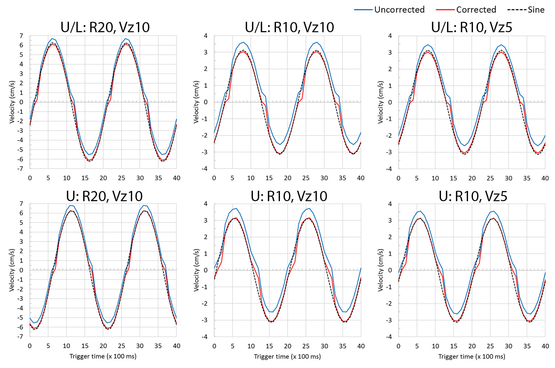
The iterative estimation of the phase offset converged sufficiently for both stationary phantom configurations as demonstrated in Figs. 3A and 3B. The two-step smoothing kernel sizes converged more than 10 times faster (Fig. 3B) than the fixed kernel size (Fig. 3A). The estimated phase offsets were spatially inhomogeneous and varied smoothly as shown in Figs. 3C and 3D. The phase offset-corrected velocities were spatially homogeneous in the flow region as shown in Fig. 4, which allowed us to use the measured velocity for the validation. The velocity curves from the phase offset-corrected velocity maps followed the driving sinusoidal movement faithfully for various motion and velocity-encoding conditions (see Fig. 5).Discussions
The only assumption of this method was that the phase offset varied slowly spatially, which was confirmed not only in this phantom study but also in the previous in vivo study.7 Therefore, the proposed method can be applied to the in vivo applications such as the CSF velocity measurement with a confidence.Conclusion
The flow phantom with the computer-controlled piston was appropriate for the validation of MR flow velocity measurement. The automated correction method of the spatially inhomogeneous phase offset was reliable and accurate in both conditions of the surrounding stationary phantom configurations and over different motion speed and velocity-encodings.Acknowledgements
No acknowledgement found.References
1. ElSankari S, et al. Concomitant analysis of arterial, venous, and CSF flows using phase-contrast MRI: a quantitative comparison between MS patients and healthy controls. J Cereb Blood Flow Metab 2013;33(9):1314-1321.
2. Hofmann E, et al. Phase-contrast MR imaging of the cervical CSF and spinal cord: volumetric motion analysis in patients with Chiari I malformation. AJNR Am J Neuroradiol 2000;21(1):151-158.
3. Bhadelia RA, et al. Analysis of cerebrospinal fluid flow waveforms with gated phase-contrast MR velocity measurements. AJNR Am J Neuroradiol 1995;16(2):389-400.
4. Walker PG, et al. Semiautomated method for noise reduction and background phase error correction in MR phase velocity data. Journal of magnetic resonance imaging : JMRI 1993;3(3):521-530.
5. Lankhaar JW, et al. Correction of phase offset errors in main pulmonary artery flow quantification. Journal of magnetic resonance imaging : JMRI 2005;22(1):73-79.
6. Jung K-J, et al. Correction of Phase Offset Induced From Eddy Current in MR Phase Contrast Cine Flow Measurement of Cerebrospinal Fluid in the Cervical Spine. Int Soc Magn Reson Med 2016.
7. Jung K-J, et al. Comparison of cervical cerebrospinal fluid flow between healthy controls and chronic spinal cord injury participants using cine phase contrast MRI. Int Soc Magn Reson Med 2016.
8. Cho ZH, et al. MR Fourier transform arteriography using spectral decomposition. Magnetic resonance in medicine : official journal of the Society of Magnetic Resonance in Medicine / Society of Magnetic Resonance in Medicine 1990;16(2):226-237.
Figures