2930
Estimating highly-accurate velocity maps from FVE MRI data using a PDE-constrained optimization1Department of Mathematics, University of Brasilia, Brasilia, Brazil, 2Engineering Faculty at Gama, University of Brasilia, Brasilia, Brazil, 3Department of Electrical Engineering, University of Brasilia, Brasilia, Brazil, 4Department of Chemical and Biomolecular Engineering, Rice University, Houston, TX, United States
Synopsis
Fourier velocity encoding (FVE) is a technique capable of delivering clinically treatable data at short acquisition times. FVE resolves the velocity distribution in each voxel of the image with high signal-to-noise ratio. This makes it suitable for the calculation of relevant biomarkers (e.g. wall shear rate and oscillatory shear index). However, it does not provide the blood flow velocity field directly. Techniques to estimate the actual blood flow from FVE velocity distributions have been previously presented. In this work, we present a novel method for velocity map estimation based on a PDE-constrained optimization that provides better results than previous methods.
Introduction
Fourier velocity encoding (FVE)[1] is an alternative to phase contrast (PC). FVE provides higher signal-to-noise ratio (SNR) than PC, due to its higher dimensionality and larger voxel sizes. FVE is robust to partial volume effects, which cause underestimation of peak-velocity in PC. FVE data are typically acquired with low spatial resolution, due to scan-time restrictions associated with its higher dimensionality. FVE resolves the velocity distribution of the spins within a large voxel, but does not directly provides a velocity map. This work proposes a novel method for estimating high-spatial-resolution velocity maps from low-spatial-resolution FVE data, based on the FVE signal model and a flow physics model.Methods
The FVE spatial-velocity distribution may be modeled as[2]: $$\hat{s\,}(x,y,v)=\left[m(x,y)\times\text{sinc}\left(\frac{v-v_z(x,y)}{\Delta v}\right)\right]\ast\psi(x,y),$$ where $$$m(x,y)$$$ and $$$v_z(x,y)$$$ are spin-density and velocity maps, respectively; $$$\psi(x,y)$$$ is the blurring kernel associated with the coverage of spatial k-space ($$$k_x$$$-$$$k_y$$$); and $$$\Delta{v}$$$ is FVE’s velocity resolution.
Blood flow can be modeled using the Navier-Stokes equation[3]: $$\rho\left(\frac{\partial\mathbf{v}}{\partial{t}}+\mathbf{v}\cdot\nabla\mathbf{v}\right)=-\nabla{p}+\mu\nabla^2\mathbf{v},$$ where $$$\mathbf{v}=(v_x,v_y,v_z)$$$ is the velocity vector; $$$\rho$$$ is the blood density; $$$\mu$$$ is the whole blood viscosity; and $$$\nabla^2$$$ is the Laplacian differential operator.
Velocity maps must (ideally) satisfy the flow physics model. Therefore, for a fixed instant of time, a velocity map can be estimated from a measured FVE dataset $$$f(x,y,v)$$$, with $$$K$$$ velocity encodes, through the following PDE-constrained optimization problem: $$\min_{v_z}\sum_{k=1}^K\int_\Omega\left\{f(\mathbf{x},v_{k})-\left[m(\mathbf{x})\times\text{sinc}\left(\frac{v_{k}-v_z}{\Delta{v}}\right)\right]\ast\psi(\mathbf{x})\right\}^2dA\,\,\,\text{s.t.}\,\,\,\rho\mathbf{v}\cdot\nabla\mathbf{v}=-\nabla{p}+\mu\nabla^2 \mathbf{v},$$ where $$$\mathbf{x}=(x,y)$$$ is the position vector, and $$$v_k$$$ is a velocity-distribution bin. In order to solve the proposed optimization, Navier-Stokes and continuity equations were discretized using the finite element method[4], as in ref. [5]. Discretized equations are written as a linear system $$$\mathbf{J}\mathbf{c}=\mathbf{r} $$$, where $$$\mathbf{J}$$$ is a matrix given by the residues' Jacobian; $$$\mathbf{r}$$$ is a vector given by the residues; and $$$\mathbf{c}$$$ is the solution vector containing velocity and pressure[4]. Then the PDE-contrained optimization problem can be written as: $$\min_{\mathbf{v}_z}\sum_{k=1}^K\left\Vert\mathbf{f}_k-\left[\mathbf{m}\times\text{sinc}\left(\frac{v_{k}-\mathbf{v}_z}{\Delta{v}}\right)\right]\ast\boldsymbol{\psi}\right\Vert_{\ell_2}^2+\lambda\left\Vert\mathbf{J}[\mathbf{v}_x;\mathbf{v}_z;\mathbf{p}]-\mathbf{r}\right\Vert_{\ell_2}^{2},$$ where $$$\mathbf{c}=[\mathbf{v}_x;\mathbf{v}_z;\mathbf{p}]$$$ is the solution vector written in a stacked form, and $$$\mathbf{m}$$$ is a spin density map with high spatial resolution.
Experiment
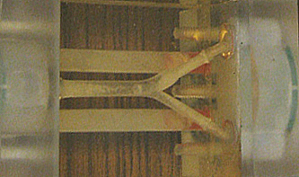
The following experiment was performed to validate the proposed method: (1) FVE data was simulated from acquired PC data; (2) the optimization was solved; (3) the resulting velocity map was compared with the acquired PC velocity map. Simulated spiral FVE data with 1 mm and 2 mm spatial resolution were derived from the through-plane velocity and spin-density maps measured using PC at the carotid bifurcation of a carotid flow phantom (Fig. 1). A 4DFT FGRE PC-MRI sequence (resolution = 1.0$$$\times$$$0.5$$$\times$$$0.5 mm$$$^3$$$, NEX = 9, VENC = 50 cm/s) was used. Lumen was manually outlined to define the computational mesh. Simulation grid was designed using $$$Q_2{}P_{-1}$$$ elements[4]. Phantom’s blood-mimicking fluid ($$$\mu$$$ = 5 mPa$$$\cdot$$$s, $$$\rho$$$ = 1100 kg/m$$$^3$$$) was assumed to be Newtonian and incompressible[3]. The discretized optimization problem was then solved using an alternating minimization technique[6]: the left-side part was solved using a standard non-linear least squares algorithm, and the physics model part was solved using Newton's method[4].Results and Discussion
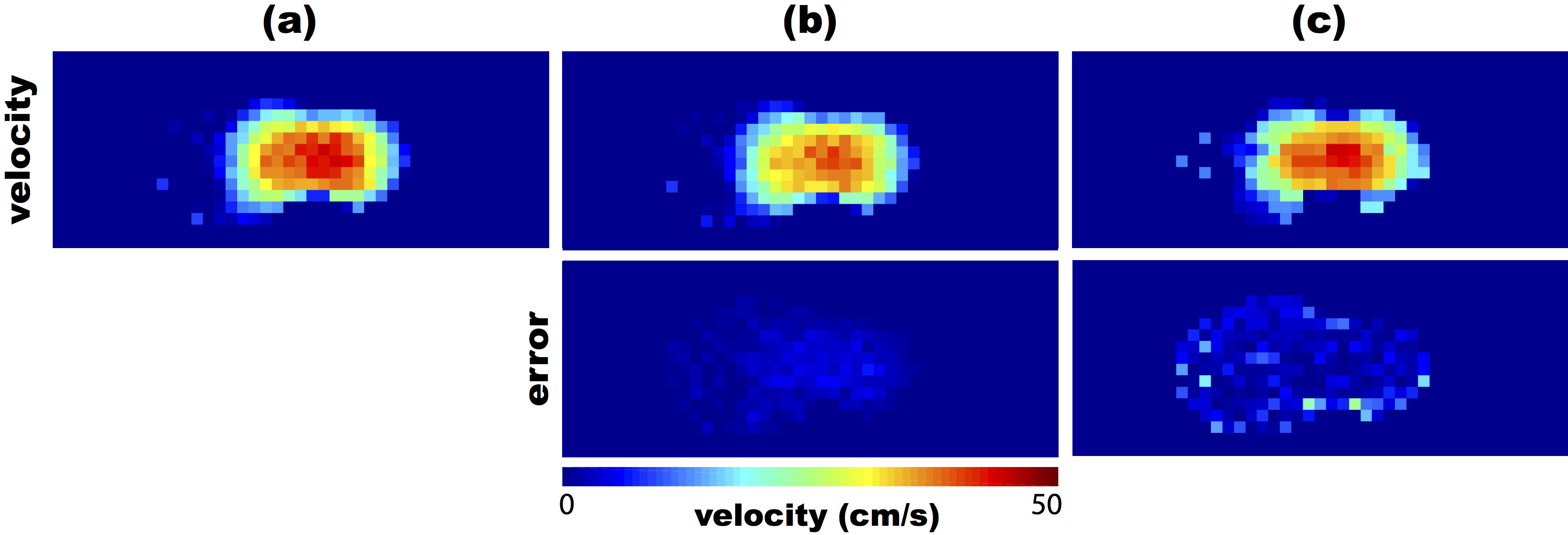
Figures 2 and 3 present the results of the validation. The velocity maps estimated from the simulated low-spatial-resolution FVE data are very similar (qualitatively) to the reference map. At first glance, one can say that the velocity maps obtained using the method from ref. [7] (Figs. 2c and 3c) are more similar to the reference velocity map. However, the error images show that the velocity maps obtained using the proposed technique (Figs. 2b and 3b) were more accurate, for both resolutions. Moreover, a quantitative comparison was performed based on the signal-to-error ratio (SER), calculated (in dB) as: $$\mathrm{SER}=10\log_{10}\left(\frac{\sum_{i,j}\left\Vert v_{\mathrm{pc}}(i,j)\right\Vert^{2}}{\sum_{i,j}\left\Vert{}v_e(i,j)-v_{\mathrm{pc}}(i,j)\right\Vert^{2}}\right),$$ where $$$v_{\mathrm{pc}}$$$ is the acquired phase contrast velocity map (used as ground-truth), and $$$v_e$$$ is the estimated velocity map. The proposed method's SERs were 50.64 dB and 44.63 dB, while the previously-proposed technique[7] achieved 32.02 dB and 28.68 dB, for 1 mm and 2 mm resolutions, respectively. This shows that the proposed method is more consistent with the actual velocity map than the previous method from the literature.Conclusion
We proposed a novel method for estimating high-spatial-resolution velocity maps from low-spatial-resolution FVE measurements. This method is based on a PDE-constrained optimization that incorporates both the FVE signal model and the Navier-Stokes equation. Results showed that it is possible to obtain highly-accurate velocity maps from FVE distributions. This means that FVE may potentially be a substitute for PC imaging, since it provides both velocity distributions and velocity map, with considerably higher SNR and robustness to partial voluming.Acknowledgements
No acknowledgement found.References
[1] Moran PR. MRI 1:197, 1982. [2] Carvalho JLA, et al. MRM 63:1537, 2010. [3] Chorin AJ and Marsden J. A Mathematical Introduction to Fluid Mechanics, 2000. [4] Gresho PM and Sani R. Incompressible Flow and the Finite Element Method, 1998. [5] Borges GB, et al. Proc ISMRM 24: 2592, 2016. [6] Wang Y, et al. SIIMS, 1:248, 2008. [7] Rispoli VC and Carvalho JLA. Proc ISMRM 21: 68, 2013.Figures