2929
4D Flow Imaging with Reduced Field-of-Excitation1Physikalisch-Technische Bundesanstalt (PTB), Braunschweig and Berlin, Germany, 2Medical Physics in Radiology, German Cancer Research Center (DKFZ), Heidelberg, Germany
Synopsis
4D flow MRI suffers from long scan times which limit maximum spatial resolutions. A promising approach is to restrict the field-of-excitation (FOX) to the region of interest and therefore reduce the field-of-view (FOV) not only in partition/slab direction, but also in phase encoding direction. In this work, we replace the slab-selective excitation of a 4D flow sequence by a 2D spatially-selective excitation with reduced FOX to enable reduced FOV imaging. We investigate the impact of the excitation on velocity encoding and demonstrate correct velocity quantification with $$$10\%$$$ reduced scan times in phantoms and in-vivo.
Introduction
4D flow MRI1 is the only technique allowing velocity vector field quantification in-vivo. However, the 3D slab-selective acquisition of the velocity vector field requires long scan times and thus limits the spatial resolution. A promising approach is to restrict the field-of-excitation (FOX) to the region of interest and therefore allow to image a reduced field-of-view (FOV) not only in partition/slab direction, but also in phase encoding direction.
In this
work, we replace the slab-selective excitation of a 4D flow sequence by a 2D
spatially-selective excitation with spiral trajectory and demonstrate correct
velocity quantification in a reduced FOX (rFOX) and reduced FOV (rFOV) in a phantom and intracranial vessels.
Methods
2D Selective Excitation
We designed a 2D selective RF-pulse with spiral k-space trajectory (Fig.1a) and bandwidth-time-product $$$\text{BWTP}=1.2$$$ in the small flip angle (FA) regime as proposed by Pauly2. The spiral starts at $$$k_{\text{max}}=2.51\,\frac{\text{rad}}{\text{cm}}$$$ and moves in $$$T=3.5\,\text{ms}$$$ with $$$n=10$$$ turns inwards to $$$\boldsymbol{k}$$$-space center.
The actual $$$\boldsymbol{k}$$$-space trajectory was measured according to Duyn3 prior to scanning (parameters: Tab.1, line1). Two RF-pulses were calculated to excite a FOX of $$$(6\times6\times\infty)\,\text{cm}^3$$$: i) based on nominal gradient waveforms (RFnom); ii) based on measured gradient waveforms (RFmeas).
4D Flow MRI Combined with 2D Selective Excitation
In order to quantify flow by phase-contrast imaging the phase of moving spins $$$\phi(v)=\gamma\,M_1\,v$$$ is manipulated by bipolar gradients such that the total first gradient moment between the effective center of excitation $$$t_0$$$ and echo-time $$$t_{\text{TE}}$$$ is $$$M_1=\int_{t_0}^{t_{\text{TE}}}G(s)\,s\,\text{d}s=\frac{\pi}{\gamma\,v_{\text{enc}}}$$$. While for symmetric SINC pulses $$$t_0$$$ is nearly at the center of the RF-pulse4, there are controversial reports about $$$t_0$$$ of 2D pulses5,6.
Therefore, we performed Bloch-simulations of our 2D spiral excitation using moving spins with varying velocities $$$v_{x,y}\in[-20,20]\,\text{m/s}$$$ to obtain the phase as a function of velocity at the end of excitation $$$T$$$. Thereby, we obtained $$$M_1^{v_i}(T)=\frac{\phi(T)}{\gamma\,v_i}$$$, where $$$i=x,y$$$. Finally, we compared it to the respective gradient moment $$$M^{v_i}_1(T) = \int_{t_0}^TG_{i}(s)\,s\,\text{d}s$$$ for $$$t_0\in[0,T]$$$.
Based on our findings, we included the 2D excitation pulse in a gradient echo 4D flow ECG-triggered MR sequence1.
Phantom and In-Vivo Experiments
Two phantom and one in-vivo measurement were performed at 3T (Magnetom Verio, Siemens, Erlangen, Germany). First, we included RFnom and RFmeas in a GRE sequence to investigate the squared excitation and non-excitation region in a large FOV using three adjacent phantom bottles (parameters: Tab.1, line2&4). To eliminate proton density and receive profiles, we normalized the data with the corresponding slab-selective acquisition (parameters: Tab.1, line3&5).
Next, the excitation performance and accuracy of flow quantification was investigated non-time-resolved in a flow phantom with constant flow. For comparison, we imaged all possible four combinations of full/reduced FOV and selective/non-selective excitation with RFmeas (parameters: Tab.1, line6-9).
Finally, a volunteer was scanned according to an approved ethical protocol and with full informed consent. A flow sequence (parameters: Tab.1, line10&11) was acquired in cerebral vessels with two different excitations targeting the Circle-of-Willis: i) 1D slab-selective excitation and ii) 2D $$$(6\times6\times\infty)\,\text{cm}^3$$$-selective excitation using RFmeas.
In all flow acquisitions, read-out was along the non-selective axis ($$$k_z$$$)
and both phase-encodings perpendicular to it. Acquisition parameters are summarized in Tab.1.
Results
Fig.1c-e show the excitation profile obtained with RFnom and RFmeas. The residual excitation of RFmeas outside the excitation window of $$$(10\times10)\,\text{cm}^2$$$ in Fig.1d is $$$(0.6\pm0.6)\%$$$.
The Bloch-simulations of moving spins show nearly velocity-independent phase at the end of the RF-pulse $$$T$$$ (Fig.2), implying $$$t_0=T$$$.
Fig.3a-d show all four combinations of 2D/non-selective excitation of the flow phantom in a full/reduced FOV. For the rFOV with non-selective excitation, biased velocities are measured, as seen quantitatively in the Bland-Altman-plot (Fig.3f). This is not seen with 2D-selective excitation (Fig.3e,g). The mean velocity difference to non-selective excitation in a full FOV is for 2D-selective excitation with full FOV $$$\Delta\,v/v_{\text{ref}}=(1.1\pm5.5)\%$$$ and with rFOV $$$\Delta\,v/v_{\text{ref}}=(2.9\pm5.9)\%$$$.
Fig.4 shows the absolute velocity and its three components during systole $$$130\,\text{ms}$$$ after ECG-trigger in the Circle-of-Willis for both 1D- and 2D-selective excitation. Qualitatively no aliasing of regions outside the FOX was observed.
Quantitatively, the flow through the internal carotids and basilar artery over the cardiac cycle is compared for both different FOXs and corresponding FOVs in Fig.4a. The maximum difference is reached during systole, $$$130\,\text{ms}$$$ after ECG-trigger, with $$$\Delta\,v/v_{\text{ref}}=6.6\%$$$.
The acquisition time with 2D excitation and rFOV was reduced by $$$10\%$$$.
Discussion and Conclusion
Here,
we demonstrate the application of a rFOX to 4D flow imaging while
correctly quantifying velocities. The present scan time reduction of only
$$$10\%$$$ is caused by the long RF-pulse duration $$$T^{RF_{\text{meas}}}=3.5\,\text{ms}>T^{\text{SINC}}=0.8\,\text{ms}$$$.
Accelerating 2D-selective excitation by parallel transmission will not only
unleash the full acceleration potential of a rFOX, but also reduce fat
sensitivity. The latter is crucial especially at ultrahigh field, which is the long-term goal of our approach.Acknowledgements
No acknowledgement found.References
1. Markl M et al. 4D flow MRI, J. Magn. Reson. Imaging 2012;36:1015-1036.
2. Pauly J et al. A k-Space Analysis of Small-Tip-Angle Excitation. J. Magn. Reson. Imaging 1989;81:43-56.
3. Duyn J H et al. Simple Correction Method for k-Space Trajectory Deviations in MRI. J. Magn. Reson. 1998;132:150-153.
4. Bernstein M A et al. Handbook of MRI pulse sequences, John Wiley & Sons, Ltd 2005
5. Hardy C J et al. Rapid NMR Cardiography with a Half-Echo M-Mode Method. J. Comput. Assist. Tomogr. 1991;15:868-874.
6. Cline H E, et al. Fast MR cardiac profiling with two-dimensional selective pulses. Magn. Res. Med. 1991;17:390-401.
Figures
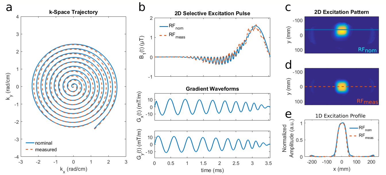
Figure 1
(a) Nominal (solid line) and measured k-space trajectory (dashed) of our 2D RF-pulse.
(b) Respective RF and gradient diagram with RF-field envelope based on nominal (RFnom, solid line) and measured gradients (RFmeas, dashed).
(c-e) Resulting excitation profile of RFnom (c, e dashed line) and RFmeas (d, e solid line).
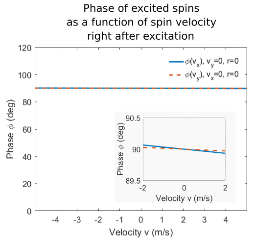
Figure 2
Phase of excited spins in isocenter as a function of spin velocity right after excitation at t=T for an exemplary pulse with spiral k-space trajectory. The inset zooms in to show the residual phase variation with velocity. The phase variation of excited spins outside the isocenter is of the same order as in isocenter.
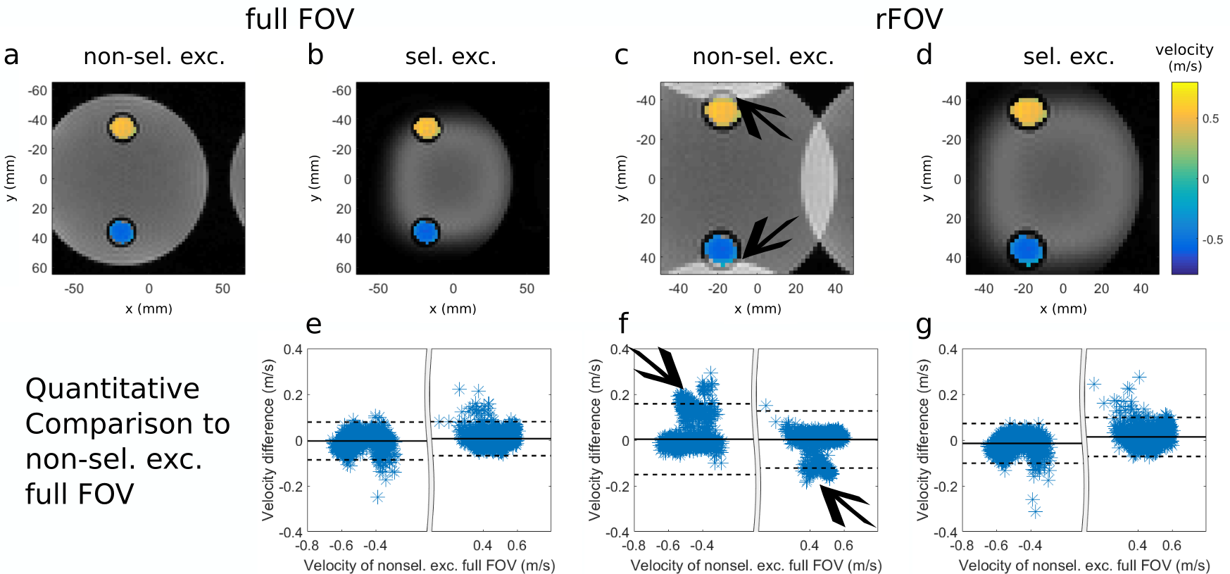
Figure 3
(a-d) Magnitude (gray) and through plane flow (colored) images of our flow phantom containing two pipes of d=10mm diameter.
(a) full FOV, non-selective excitation, (b) full FOV, selective excitation, (c) rFOV, non-selective excitation, and (d) rFOV, selective excitation.
(e-g) Bland-Altman plots of the velocities quantified within the pipes corresponding to images (b-d) compared to full FOV, non-selective excitation. Solid lines indicate the mean velocity deviation and dashed lines the three-fold standard deviation.
Arrows indicate where signal from non-selectively excited spins is aliased into the rFOV, which results in biased velocity quantification.
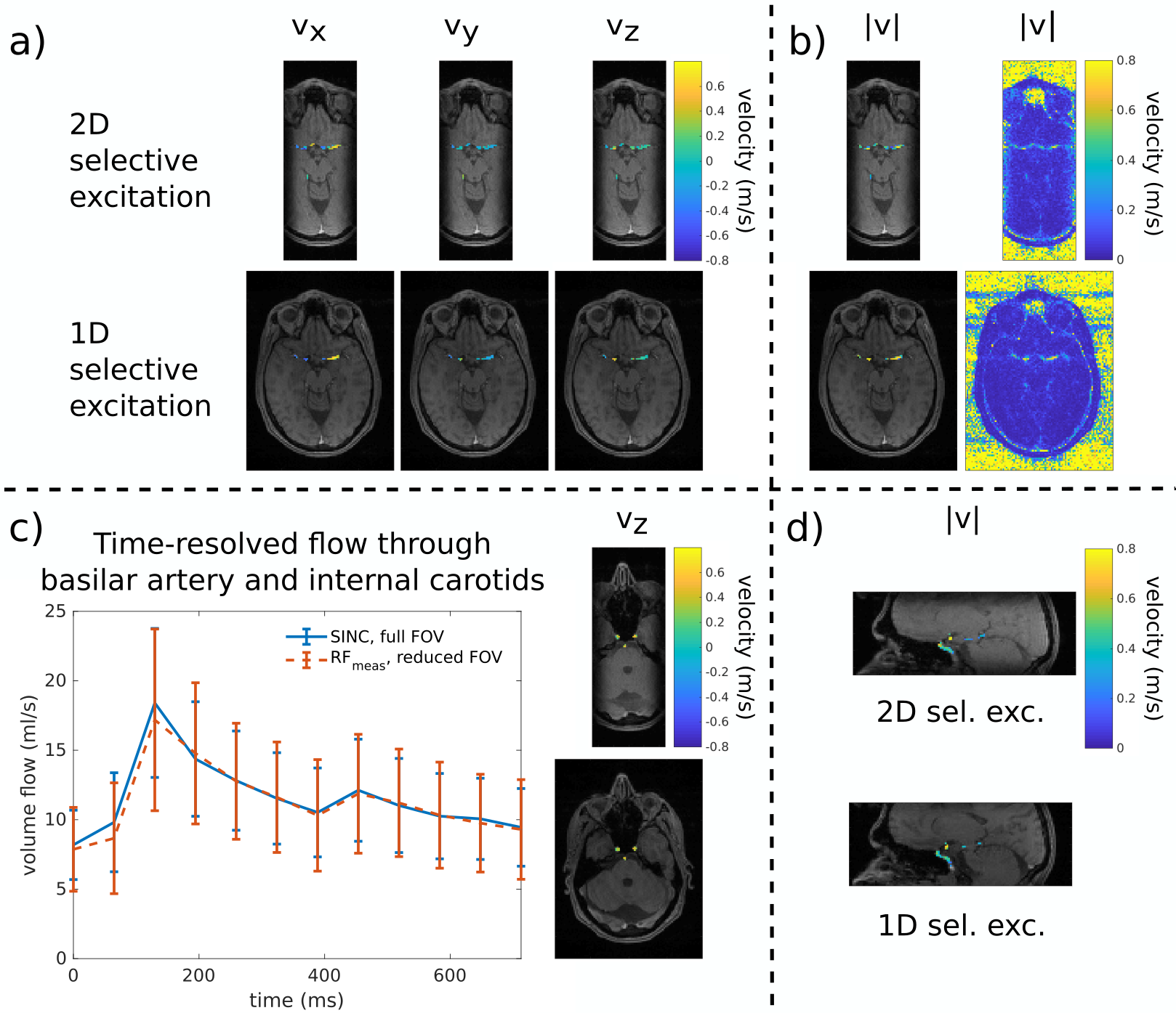
Figure 4
(a-b,d) Comparison of GRE magnitude (gray-scale) and velocity images (color-coded) between 1D- (bottom row) and 2D-selective excitation (top row) in the Circle-of-Willis during systole, 129.6ms after ECG-trigger.
(c) Comparison of time-resolved flow through the basilar artery and internal carotids between a full FOX/FOV- (solid line) and a rFOX/rFOV-acquisition in PE-direction (dashed line). The error bars are the standard deviation of all 37 voxels of the basilar artery and internal carotids including the physiological velocity profile. The figures on the right show a respective slice of a full FOX/FOV-acquisition (bottom) and rFOX/rFOV-acquisition (top).
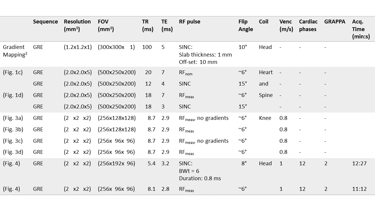
Table 1
Table of acquisition parameters.
For the RF-pulses RFmeas & RFnom the given flip angles are nominal flip angles. If no number of cardiac phases is given, the scan is time-unresolved. The given acquisition time is a nominal value for an acquisition window of 778ms.