2864
A Principled Approach to Combining Inversion Recovery Images1Department of Biomedical Engineering, University of Basel, Allschwil, Switzerland, 2Division of Radiological Physics, Department of Radiology, University Hospital Basel, Basel, Switzerland, 3Department of Neurology, University Hospital Basel, Basel, Switzerland
Synopsis
The averaged magnetization inversion recovery acquisitions (AMIRA) spinal cord imaging sequence acquires images of different inversion contrasts. Despite the different contrasts the images can be combined to even enhance tissue contrast. We give a principled justification for such averaging. Using energy optimization, we describe how to automatically optimize the contrast-to-noise ratio between different tissues using a compressed sensing inspired approach. We show that the uniform weights in the recently proposed AMIRA sequence are close to the optimum but can nevertheless still be improved. As an example we optimize the contrast-to-noise ratio between different compartments in the spinal cord.
Purpose
Recently, a fast high-resolution spinal cord imaging sequence with averaged magnetization inversion recovery acquisitions (AMIRA) has been presented [1]. This sequence acquires 8 images at different inversion times, whose average gives better contrast-to-noise ratio. The original work proposes to average the first 5 images for optimal spinal cord gray matter (GM) and white matter (WM) contrast and to average the last 5 images for optimal WM and cerebrospinal fluid (CSF) contrast. Direct averaging of some of the acquired images is a promising but still simple concept. In the following we analyze whether a non-uniform averaging could improve the contrast. Using energy minimization, we calculate coefficients for optimal linear combinations of the 8 inversion images with best contrast-to-noise ratios.Method
We present an energy functional, which is based on the idea of compressed sensing [2]. Given some images $$$I_1,\ldots,I_n$$$, with values between 0 and 1, we search for coefficients $$$c = (c_1,\ldots,c_n)$$$ where the linear combination $$$I(c) := c_1 \cdot I_1 + \ldots + c_n \cdot I_n$$$ yields an optimal contrast-to-noise ratio. Suppose we have a manual segmentation of tissue $$$A$$$ and $$$B$$$ (subsets of the image domain) and suppose tissue $$$A$$$ has bright intensities close to 1 and tissue $$$B$$$ has dark intensities close to 0 (or at least darker than tissue $$$A$$$). We define the energy $$\begin{align}\mathscr{E}(c) := &\,\, \lambda_1 \frac{\sum_{x\in A} (I(c)(x)\, – 1)^2 }{|A|} + \lambda_2 \frac{\sum_{x\in B} (I(c)(x))^2 }{|B|} \,\,+ \\\\ & - \lambda_3 \big| E[I(c)(A)]-E[I(c)(B)] \big| + \lambda_4 V[I(c)(A)] + \lambda_5 V[I(c)(B)] \,\,+ \\\\ &- \lambda_6 \sum_{k=1}^n c_k \big| E[ I_k(A) ]-E[ I_k(B)] \big|+ \lambda_7 \sum_{k=1}^n c_k V[I_k(A)] + \lambda_8 \sum_{k=1}^n c_k V[I_k(B)] \,\,+ \\\\ &+ \lambda_9 \mathcal{R}(c),\end{align}$$ where $$$|A|$$$ is the cardinality of $$$A$$$, $$$I(A)$$$ is the set of all intensities of tissue $$$A$$$ on an image $$$I$$$, and $$$E[I(A)]$$$ and $$$V[I(A)]$$$ is the mean and variance of the intensities of tissue $$$A$$$ on an image $$$I$$$, respectively. The first two summands in $$$\mathscr{E}$$$ encourage the linear combination $$$I(c)$$$ to be as close to the segmentation as possible, the third negative term maximizes the contrast, and the fourth and fifth terms minimize noise. Terms 6, 7 and 8 in the third line also maximize contrast and minimize noise, however on the level of the individual inversion images. With the regularization $$\mathcal{R}(c) := \left( 1-\sum_{k=1}^n |c_k|\right)^2,$$ we weakly constrain the coefficients’ absolute values to sum up to 1. This way we omit arbitrarily large coefficients and we enable meaningful negative coefficients. A negative coefficient $$$c_k$$$ flips the contrast of an inversion image $$$I_k$$$ between tissue $$$A$$$ and $$$B$$$. $$$\mathscr{E}$$$ is minimized using BFGS.
We optimized the coefficients for a total of 68 slices on 4 different subjects at different vertebral heights (C2-C5) acquired with the AMIRA sequence. For each slice, we calculated linear coefficients $$$c_{\text{CSF/WM}}$$$ for optimal CSF/WM contrast and another set of linear coefficients $$$c_{\text{GM/WM}}$$$ for optimal GM/WM contrast, see Figure 2 and 3.
Results and Discussion
Figure 1 shows a representative series of the 8 images acquired by the AMIRA sequence and the suggested optimized CSF/WM and GM/WM contrast averages of an exemplary single axial slice located at level C2-C3. The optimized coefficients and their statistics are shown in Figure 2 and 3. The calculated optimal coefficients for GM/WM and for CSF/WM contrast are similar to uniform averaging, but they also address the weaker signal of inversion images at later inversion times, e.g. the drop of $$$c_8$$$ in Figure 2. For the calculated CSF/WM coefficients, we may now include the first inversion image, which has darker CSF and brighter WM, by allowing negative coefficients $$$c_k$$$. A flipped image $$$c_k \cdot I_k$$$ can be combined with the inversion images $$$I_5$$$ to $$$I_8$$$, where the CSF is brighter than WM. We empirically have chosen $$$\lambda_1,\ldots,\lambda_9$$$ to be 100, 100, 1, 1, 1, 10, 10, 10, and 1000, respectively.
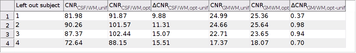
For quantitative comparison we calculated contrast to noise ratios $$$\text{CNR}_{A/B}=\text{SNR}_{A}-\text{SNR}_{B}$$$ and signal to noise ratios $$$\text{SNR}_{A}=E[I(A)] \big/ SD[I(C)]$$$. We estimated the standard deviation of noise $$$SD[I(C)]$$$ on a homogeneous part $$$C$$$ of the background. Figure 4 shows a quantitative comparison of CNR between uniform and proposed averaging. Leave-one-subject-out results are shown in Figure 5.
Conclusion
With the proposed method we analyze the uniform averaging technique of the inversion images of the AMIRA sequence. The found calculated coefficients are close to the uniform coefficients and the contrast-to-noise ratios can slightly be improved. For CSF/WM contrast a notable improvement was possible. With the developed approach, we could justify the decisions made in [1] on a quantitative basis. The optimization coefficients can be chosen for the needs, e.g. prioritizing less noise or better contrast.
Acknowledgements
This work was supported by the Swiss National Science Foundation (SNF grant No. SNF 320030-156860/1).References
[1] Weigel M, Bieri O. Spinal cord imaging using averaged magnetization inversion recovery acquisitions. Magn Reson Med 2017 Jul 16. doi: 10.1002/mrm.26833.
[2] D. L. Donoho. Compressed sensing. IEEE Transactions on Information Theory, vol. 52, no. 4, pp. 1289–1306, Apr. 2006.
Figures
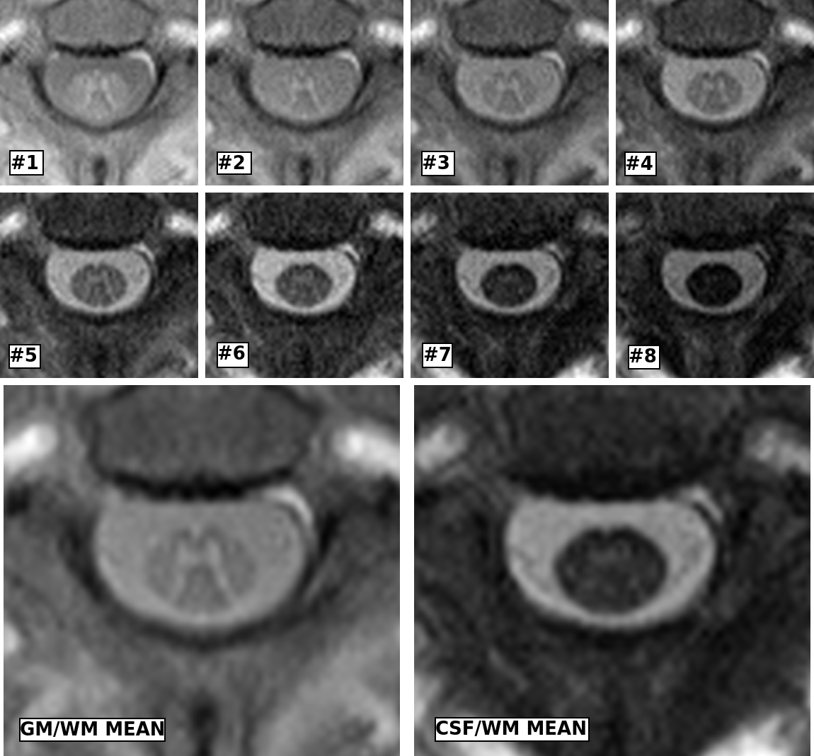
Figure 1: Top and middle row: series of the 8 acquired inversion images of the AMIRA sequence in chronological acquisition order from top left to bottom right (zoomed in and upsampled). Bottom row: resized CSF/WM and GM/WM averages of the AMIRA images (combined with the mean coefficient values of Figure 2 and Figure 3, respectively).
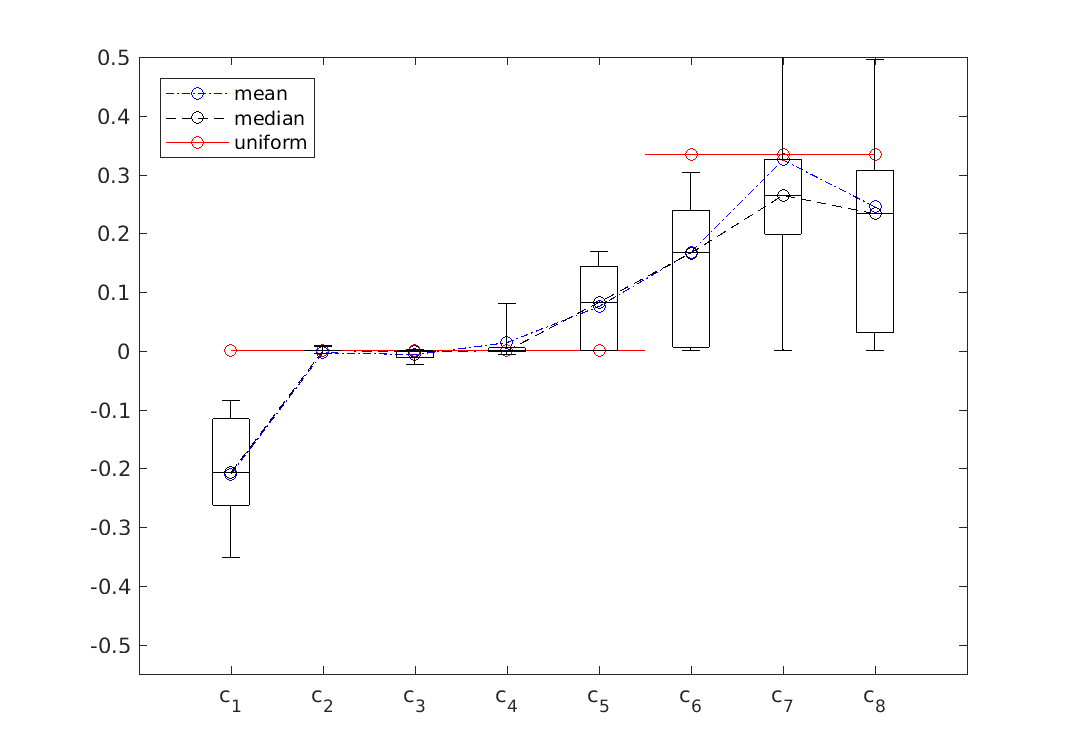
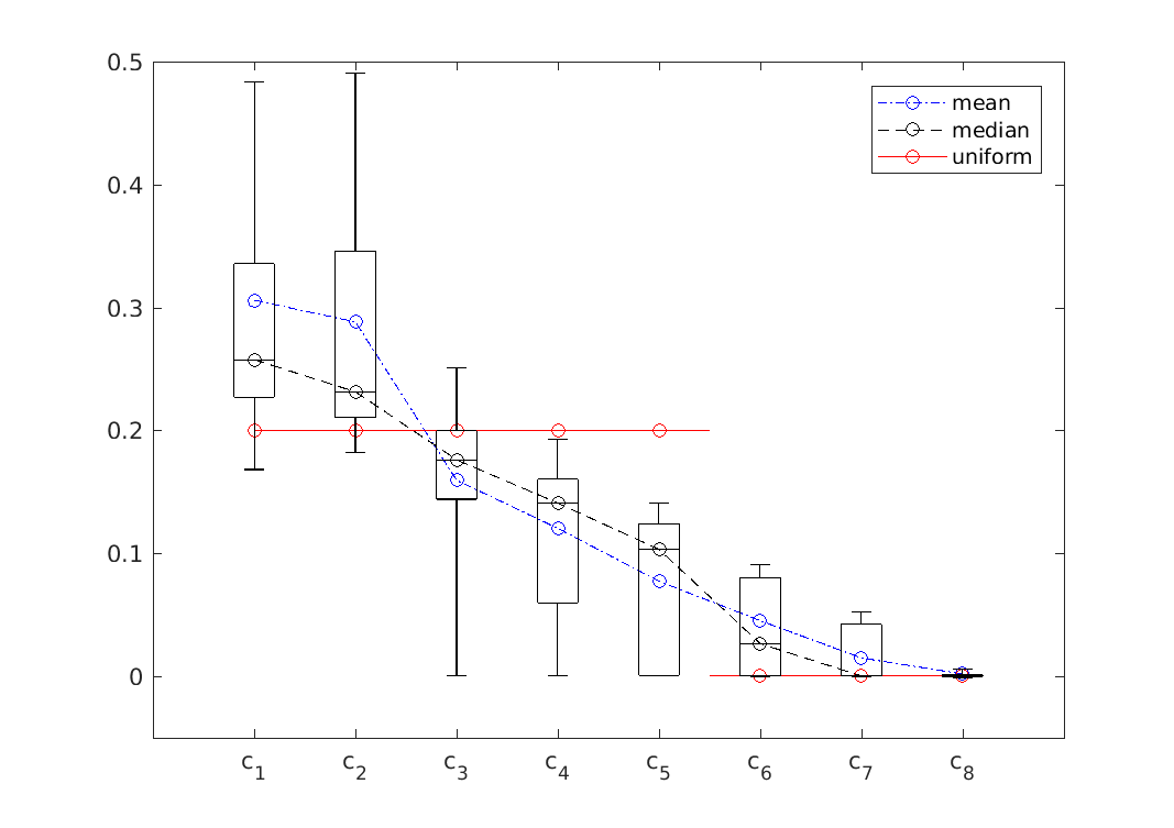
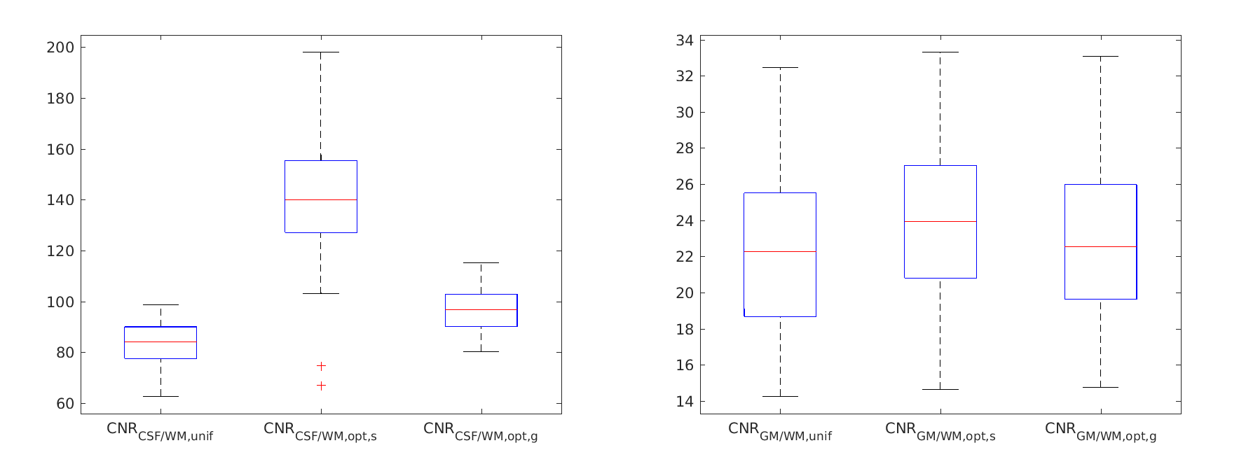
Figure 4: Contrast-to-noise ratios, comparing the uniform averaging (unif) and the optimized coefficients (opt). The optimized coefficients are evaluated for two cases: the optimal case (s), where the optimal coefficients $$$c$$$ of each slice were used to calculate the linear combination $$$I(c)$$$ for each slice; and the global case (g), where the blue mean value coefficients of Figure 2 and 3, respectively, were used for all slices. Left: CNR comparison for CSF/WM contrast enhancement; right: comparison for GM/WM contrast enhancement.
Mean values from left to right: 83, 139, 97, 22, 24, 23.