Synopsis

Medical imaging core lab centres face increasing quality control (QC) challenges as studies/trials become larger and more complex. Many QC processes are performed manually by experts, a time-consuming process. Most of the work on automated medical image QC in the literature focuses on text-based metadata correction, thus automated QC algorithms that are able to detect inconsistencies with image data only are needed. We propose two different methods for classification of anonymized MR images by acquisition method (T1-w, T2-w, T1 post contrast, or FLAIR). The classifiers were trained on the MICCAI-BRATS 2016 dataset and achieved accuracies of 85.7% and 93.8%.

Introduction

Quality control (QC) has become essential as imaging studies grow in size, variability and complexity. QC correction of text-based data is somewhat straightforward with current technologies. However, this ability is not true for imaging data, where these processes rapidly become extremely resource intensive. Many QC processes are performed manually, through standardization of image acquisition, or by experts performing hands-on review of acquired images prior to inclusion in the repositories. Improved approaches to QC that are more cost-effective and account for data heterogeneity in imaging studies are needed.

There are many approaches to achieve quality in imaging repositories¹ with recent efforts focusing on techniques to automatically identify images of poor quality (e.g., excessive noise, motion or other artifact).^2,3 However, variations in modality, acquisition parameters and incomplete metadata contribute to data heterogeneity, requiring expert hands-on review for such tasks. There is a need for computer-assisted techniques that classify and sort images based on their contrast or acquisition characteristics. We propose and compare two machine learning (ML) techniques to identify MR images of different sequences by using only image information. These methods may be used to complete missing MR information or to verify protocol compliance of an imaging dataset.

Methods

We implemented two different methods for MR sequence classification: ML1) a traditional ML classifier with hand-crafted texture features; and ML2) a convolutional neural network (CNN) with ten layers and end-to-end classification. Performance was evaluated by the accuracy rate of the two classification methods.

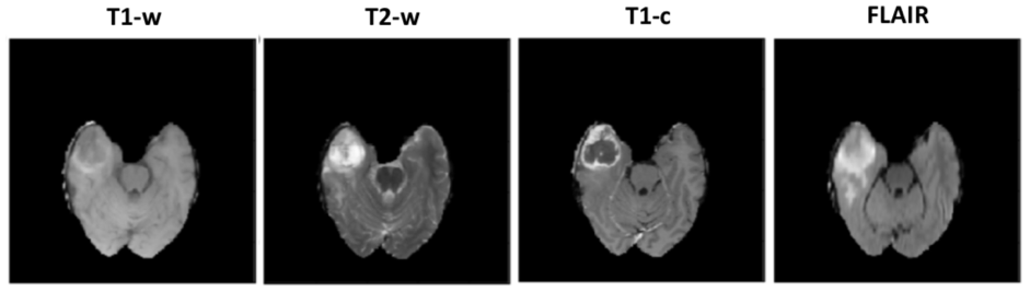
The MICCAI-BRATS 2016 dataset, comprising MR brain scans from 274 patients with low- or high-grade glioblastoma, was used to train the classifiers. For each patient, four three-dimensional (3D) volumes are available, corresponding to different sequence: T1-weighted (T1-w), T2-weighted (T2-w), T1 post-contrast (T1-c) and fluid attenuated inversion recovery (FLAIR). Each volume has a resolution of 240×240×140 and the images were originally registered to the other sequence scans and skull-stripped (Figure 1). All scans were first normalized to standardize their intensity within the range [0,255].

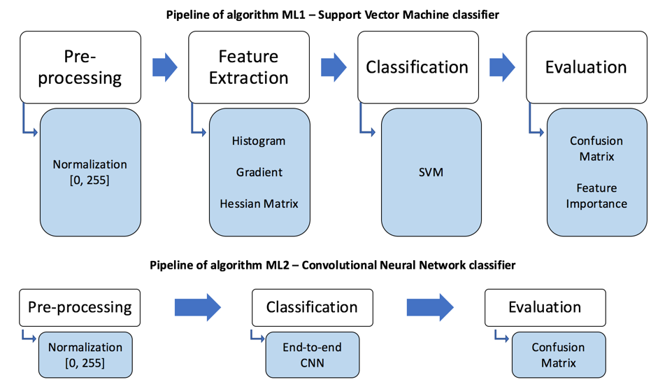
ML1 used a support vector machine (SVM) model to build a classifier (Figure 2). Hand-crafted texture features were extracted including statistics from the grayscale histogram; the grayscale gradients (in 3 orthogonal directions); and the mean values of the Hessian matrices (6 directions).⁴ The data was split into training and testing sets using 5-fold cross-validation.⁵ The SVM parameters were optimized using grid search.⁶ Degree of feature importance was then determined using random forests.⁷

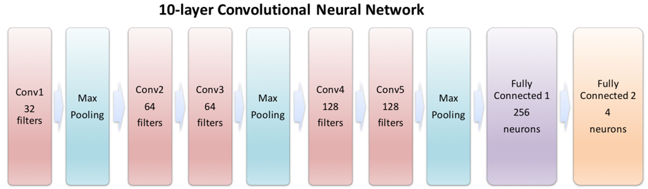
ML2 had a ten-layer deep CNN architecture (Figure 3). For training, each slice of the 1,096 volumes was used as an independent input (rather than using the entire 3D volume). The adjusted dataset containing 4×274×140 = 153,440 240×240 axial labeled images was partitioned; 70% for training, 30% for testing.

Results

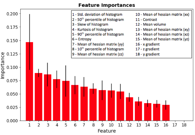
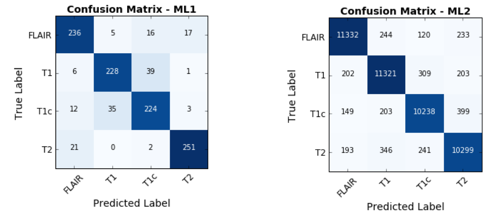
The ML1 algorithm achieved an accuracy of 85.7% using a linear kernel and C=10 on the 1,094-element scan volume dataset. The most discriminant feature was the standard deviation of the pixel intensity histogram (Figure 4). Training time was 3 minutes and testing time 66 ms on a computer with a first-generation Intel Core i7. The ML2 algorithm achieved an accuracy of 93.8% on the 46,032-element two-dimensional testing dataset. Training time was 8 hours and testing time was 93 ms on the same computer.

Discussion

Our results demonstrate that training a deep classifier (ML2) for MR sequence classification results in a higher accuracy than using a more conventional classifier (ML1). However, training time is considerably higher. This result was expected as the number of parameters learnt by the ML2 architecture is much larger.

It is important to consider that the two classifiers were trained to perform slightly different tasks. As the ML2 classifies on a slice-by-slice basis, it may be possible to generate a functionally equivalent classifier by using the consensus between the classification of all slices. Because the classifiers were not trained on a heterogenous MR dataset, they may not be as accurate in classifying brain MR images without gliomas.

Conclusion

Acknowledgements

References

1 - Gorgolewski KJ, Auer T, Calhoun VD, Craddock RC, Das S, Duff EP, et al. The brain imaging data structure, a format for organizing and describing outputs of neuroimaging experiments. Scientific Data 2016; 3: 160044.

2- Quality control. NIH MRI Study of Normal Brain Development - Quality Control. http://www.bic.mni.mcgill.ca/nihpd/info/quality_control.html#MRIQC. Accessed November 02, 2017

3- Gedamu EL, Collins D, Arnold DL. Automated quality control of brain MR images. Journal of Magnetic Resonance Imaging 2008; 28: 308–19.

4- Gonzalez RC, Woods RE. Digital image processing. Pearson; 2002.

5- Kohavi, R. A Study of Cross-Validation and Bootstrap for Accuracy Estimation and Model Selection [PDF]. Retrieved from: http://robotics.stanford.edu/~ronnyk/accEst.pdf. 1995.

6- Bergstra, J., & Bengio, Y. . Random search for hyper-parameter optimization. Journal of Machine Learning Research 2012; 13: 281-305.

7- Brieman, L. . Random forests. Machine Learning 2001; 45: 5-32.