2833

A Comparison of Brain Subnetwork Extraction Methods

Elizabeth Ceiridwen Anne Powell^1,2, Ferran Prados^2,3, Baris Kanber^2,3, Wallace Brownlee², Sara Collorone², Sebastien Ourselin³, Olga Ciccarelli², Jonathan D Clayden⁴, Ahmed Toosy², and Claudia Angela Gandini Wheeler-Kingshott²

¹Medical Physics and Biomedical Engineering, University College London, London, United Kingdom, ²Queen Square MS Centre, UCL Institute of Neurology, Faculty of Brain Sciences, University College London, London, United Kingdom, ³Translational Imaging Group, Centre for Medical Image Computing, Medical Physics and Biomedical Engineering, University College London, London, United Kingdom, ⁴Developmental Imaging and Biophysics Section, Great Ormond Street Institute of Child Health, University College London, London, United Kingdom

Synopsis

In the complex network model of the brain it is often noted that a subset of nodes, or subnetwork, plays a central role in network architecture, whose damage could have a disproportionate effect on network resilience to injury. The identification of "important" nodes in a network is non-trivial though, and several fundamentally different methods exist; it is currently unclear to what extent these methods agree. In this work we demonstrate that subnetworks extracted using rich club and principal network analysis share 60% of nodes, suggesting a core subset of nodes are important to network architecture independently of analysis model.

Introduction

In the complex network model of the human brain, it is often noted that a subset of nodes plays a central role in network architecture^1,2. Hub nodes, for example, exhibit high degree properties, and are thus important for network integration; however, local damage to hub nodes may have a disproportionate effect on network resilience to injury.

The "rich club" phenomenon proposes a description in which hub nodes are densely interconnected with fewer connections to lower degree nodes. The regions that form these rich clubs can be classified as a subnetwork, offering high communication efficiency and some level of network resilience to the failure of a hub node.

The identification of "important" nodes in a network is non-trivial though, and there exist alternative methods of extracting salient regions. Recently, the concept of principal networks³ was introduced. Principal network analysis (PNA) involves the eigendecomposition of the association matrix, $\bf{A}$ , into its canonical form ( $\bf{A}=\bf{Q \Lambda Q}^{-1}$ ). The eigenvector element $Q_{ij}$ , or loading, represents the influence of node $i$ on principal network (PN) $j$ . PNs are subsequently formed from nodes with similar connectivity properties.

In this work we examine the agreement between two independent techniques, namely rich club analysis and PNA, used for extracting subnetworks based on key nodes from cortical thickness data.

Methods

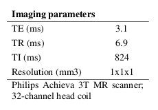
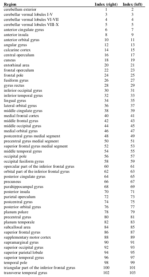
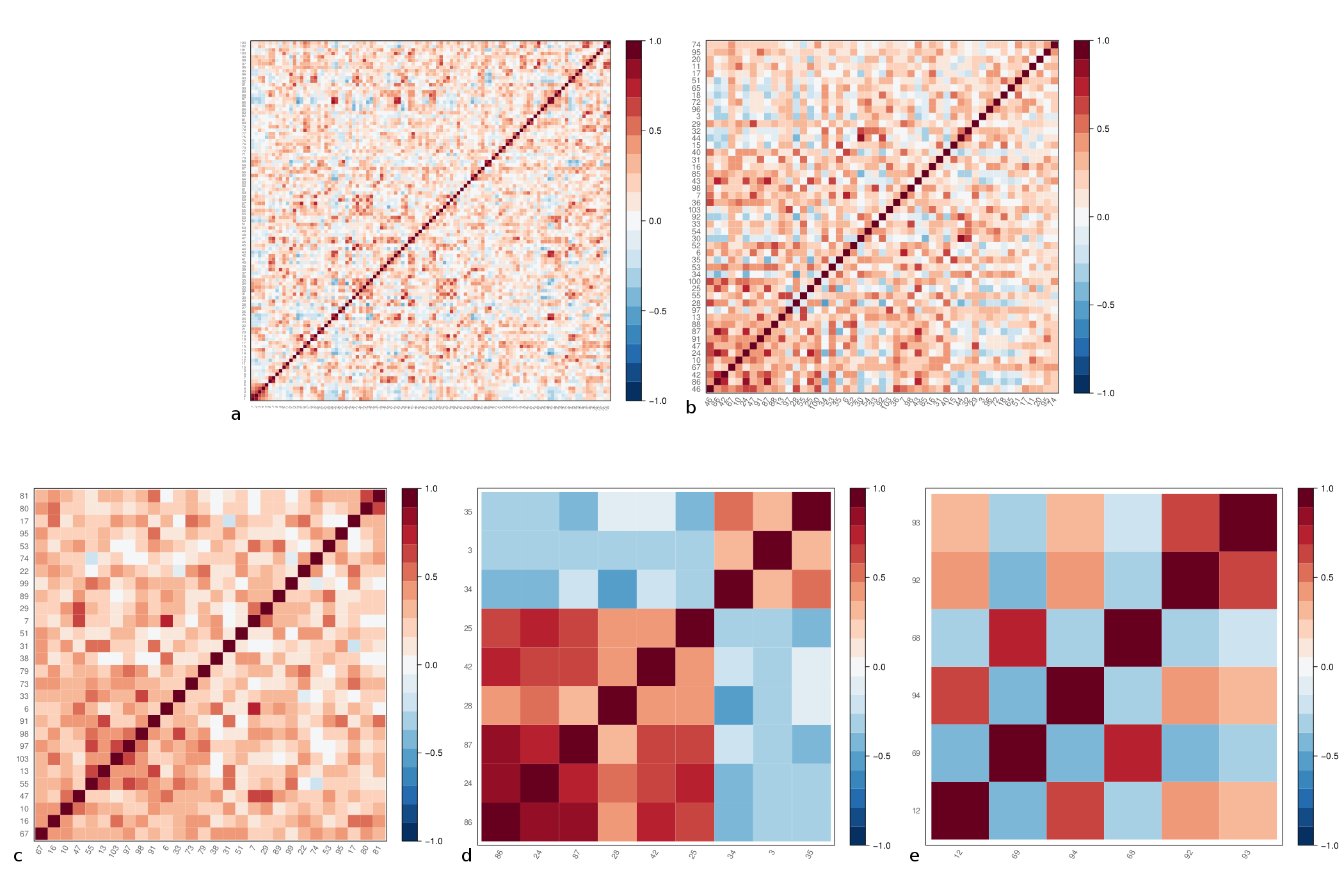
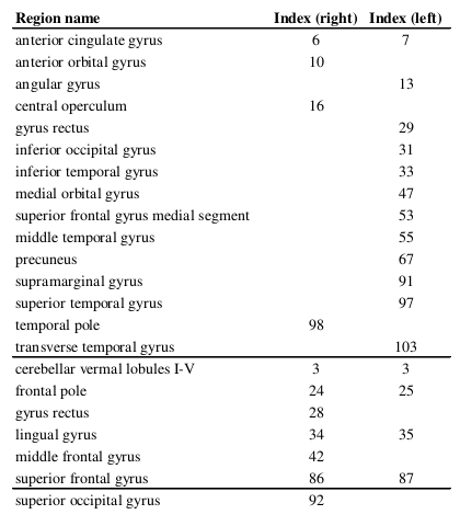
T₁-weighted images were acquired on 46 healthy controls (26 females; mean age 34 ± 8.6 years); imaging parameters and hardware specifications are given in Figure 1. The thickness of $N=103$ parcellated^4,5 cortical regions was computed⁶; correspondences between cortical region indices and anatomical names are given in Figure 2. An association matrix, or network, $\bf{A}$ , was generated using correlations in cortical thickness (Figure 3a).

Subnetworks defined using PNA, $S_{pna}^j$ , were generated such that $\vert Q_{ij} \vert>0$ , with $i=\left\{ 1,…,N \right\}$ and $j=\left\{ 1,2,3 \right\}$ , at 5% significance level, as determined from 1000 bootstrapped samples of $\bf{A}$ with replacement. Nodes were ranked according to loading magnitude.

For the rich club subnetwork, $S_{rc}$ , normalised weighted rich club coefficients $\phi_{norm}\left(k\right)$ ¹ were generated over the degree range $1<k<k_{max}$ , where $k_{max}$ was the maximum nodal degree in $\bf{A}$ . Normalisation was performed using the rich club coefficient averaged over 1000 randomly generated networks⁷. The subnetwork was defined from the nodes that formed the most selective rich club (greatest possible degree threshold) within the rich club regime, defined by the range of $k$ in which $\phi_{norm}\left(k\right)>1$ and is increasing. Nodes were ranked according to their strength in $S_{rc}$ .

Results

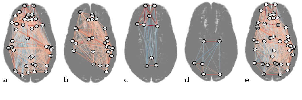
Figures 3b-e and 4a-e display the derived subnetworks. Subnetwork $S_{pna}^1$ was dominated by nodes with strong positive edges, while nodes with positive and negative edge weights featured in $S_{pna}^2$ , $S_{pna}^3$ and $S_{rc}$ .

Comparing the nodes in subnetworks $S_{pna}^1$ , $S_{pna}^2$ and $S_{pna}^3$ with $S_{rc}$ we find that: 71% of $S_{pna}^1$ nodes featured in $S_{rc}$ ; 100% of $S_{pna}^2$ nodes featured in $S_{rc}$ ; 17% of $S_{pna}^3$ nodes featured in $S_{rc}$ . Of the 43 nodes in subnetworks $S_{pna}^1$ , $S_{pna}^2$ and $S_{pna}^3$ combined, there was 60% agreement with the highest ranked 43 nodes in $S_{rc}$ (Figure 5).

Discussion

Several nodes common to $S_{rc}$ and $S_{pna}^1$ , such as the precuneus, angular gyrus and temporal gyri, correspond to core regions of the default mode network (DMN), which is formed of highly interconnected areas likely to contain hub nodes² with similar connectivity properties. Nodes unique to individual subnetworks were defined by the analysis technique: nodes similarly connected by strong positive correlations were retained in $S_{pna}^1$ , while in $S_{rc}$ positive and negative correlations were retained because both can feature in hub nodes. The primarily anti-correlated nodes in $S_{rc}$ notably appeared in the lower order PNs $S_{pna}^2$ and $S_{pna}^3$ , reflecting the characteristic property of PNA to group together nodes with similar connectivity attributes.

A limitation on the generation of subnetworks using either technique was their inherent dependency on the inclusion criteria for salient nodes. Bootstrapping the association matrix in PNA provided a more statistically robust set of nodes compared to the simple threshold proposed in the original method³. The degree threshold applied in rich club analysis affected the subnetwork size and therefore the featured anatomical regions; future studies could evaluate subnetworks generated over a range of degree thresholds within the rich club regime.

Conclusions

Subnetworks created using two unrelated techniques for identifying nodes influential in overall network characteristics shared 60% of their 43 highest ranked nodes, several of which belong to the DMN. This suggests that there is a core subset of nodes that are important independently of how “importance” is modelled. The remaining nodes unique to each subnetwork ultimately depend on the biophysical meaning of the analysis technique.

Acknowledgements

Horizon2020-EU.3.1 (ref: 634541). UK MS Society. NIHR Biomedical Research Centres (BRC R&D03/10/RAG0449).

References

Sporns O, Honey C, Kötter R. Identification and classification of hubs in brain networks. PLoS One. 2007;2(10).
van den Heuvel MP, Sporns O. Rich-Club Organization of the Human Connectome. J Neurosci. 2011;31(44):15775-15786.
Clayden JD, Dayan M, Clark CA. Principal Networks. PLoS One. 2013;8(4):1-12.
Cardoso MJ, Modat M, Wolz R, et al. Geodesic information flows: spatially-variant graphs and their application to segmentation and fusion. IEEE Trans Med Imaging. 2015;34(9):1976-1988.
Prados F, Cardoso MJ, Burgos N, Angela C, Gandini M, Ourselin S. NiftyWeb : web based platform for image processing on the cloud. In: International Society for Magnetic Resonance in Medicine (ISMRM) 24th Scientific Meeting and Exhibition, Singapore. Singapore; 2016.
Tustison NJ, Cook PA, Klein A, et al. Large-scale evaluation of ANTs and FreeSurfer cortical thickness measurements. Neuroimage. 2014;99:166-179.
Rubinov M, Sporns O. Complex network measures of brain connectivity: Uses and interpretations. Neuroimage. 2010;52(3):1059-1069.

Figures

MR acquisition parameters.

Correspondences between node indices and anatomical brain regions.

Matrix visualisations of the networks and subnetworks; the colourbar represents Pearson’s correlation coefficient between nodes. Nodes in subnetworks b-d are ranked, with the most “important” bottom left. a). Full association network A, containing 103 parcellated cortical regions; b). Subnetwork

$S_{rc}$ , with 47 nodes; c). Subnetwork

$S_{pna}^1$ , with 28 nodes; d). Subnetwork

$S_{pna}^2$ , 9 nodes; e). Subnetwork

$S_{pna}^3$ , 6 nodes. Subnetwork

$S_{pna}^1$ is dominated by strong positive connections; subnetworks

$S_{pna}^2$ ,

$S_{pna}^3$ and

$S_{rc}$ contain both positively and negatively correlated nodes.

Graphical representation of nodes in each subnetwork. Edge colours represent Pearson’s correlation coefficient between nodes: deep red (blue) edges denote strong positive (negative) correlations. Image orientation follows the radiological convention (image top left is brain anterior right). a). Subnetwork

$S_{rc}$ , highest ranked 43 nodes; b). Subnetwork

$S_{pna}^1$ ; c). Subnetwork

$S_{pna}^2$ ; d). Subnetwork

$S_{pna}^3$ ; e). Combined subnetworks

$S_{pna}^1$ ,

$S_{pna}^2$ and

$S_{pna}^3$ , 43 nodes.

Anatomical regions common to

$S_{pna}^1$ and

$S_{rc}$ (top set), to

$S_{pna}^2$ and

$S_{rc}$ (middle set), and to

$S_{pna}^3$ and

$S_{rc}$ (bottom set). It is interesting to note the laterality of the common regions between

$S_{pna}^1$ and

$S_{rc}$ . It is possible that this is explained in part by PNA identifying salient nodes in the dominant hemisphere of the primarily right-handed cohort.

Proc. Intl. Soc. Mag. Reson. Med. 26 (2018)

2833