Synopsis

We propose a new tool in AFNI-FATCAT to estimate the above RSFC parameters even when time series are censored, using the Lomb-Scargle (L-S) periodogram. The L-S approach for estimating RSFC parameters is useful and generalizable for FMRI data, where censoring is nearly always performed during processing. The method shows minimal bias of parameter estimation, and also allows for the estimation of confidence intervals for the parameters.

Introduction

Methods

The Lomb-Scargle (L-S) periodogram was developed to examine periodicity in non-uniformly sampled time series [4-5]. Here, we use the efficient form of L-S calculation from [6], whose results in the presence of no censoring exactly match those from FFT, so the L-S approach can be applied generally. We assume the time series have been de-meaned, with either no or non-uniform (i.e., approximately random) censoring. Amplitudes are calculated up to a maximum frequency (pseudo-Nyquist limit), with an appropriate value shown to be $$$f_{max} = 1/(2*TR)$$$, where TR is sampling rate of acquisition [6]; with no censoring, this upper frequency precisely matches with the FFT case (the Nyquist limit). In traditional (uncensored) calculations, the ALFF and RSFA parameters from a (zero mean) time series $$$x_n$$$ of $$$N$$$ time points can be expressed as a sum of spectral amplitudes $$$|X_k|$$$ with harmonics in the interval $$$k\in[A, B]$$$: $$RSFA=\sqrt{\frac{1}{(N-1)N}\sum_{k=A}^{B}|X_k|^2}\,,~~~~~~~~ALFF=\frac{1}{\sqrt{N}}\sum_{k=A}^{B}|X_k|\,.$$ When censoring, the forms and scaling of the RSFC quantities must be expressed so the parameters are unbiased with respect to the the number of censored time points. Here, we derive the quantities starting from Parseval’s theorem, a standard relation between $N$ time points $x_n$ (here, with zero mean) and their $L = N/2$ independent spectral amplitudes $|X_k|$:

$$\sum_{n=0}^{N-1}|x_n|^2=\frac{1}{N}\sum_{k=0}^{N-1}|X_k|^2\,.$$

For real-valued, zero-mean time series, symmetries in the spectrum lead to:

$$\sum_{n=0}^{N-1}|x_n|^2=\frac{1}{L}\sum_{k=1}^{L-1}|X_k|^2\,.$$

These relations can be expressed with reference to the definition of variance:

$$\sigma^2=\frac{1}{N-1}\sum_{n=0}^{N-1}|x_n|^2=\frac{1}{(N-1)L}\sum_{k=1}^{L-1}|X_k|^2\,.$$

RSFA is the standard deviation of the LFF-bandpassed time series $$$x’_n$$$ with frequency harmonics in the interval [A, B]: $$RSFA^2=\frac{1}{N-1}\sum_{n=0}^{N-1}|x’_n|^2=\frac{1}{(N-1)L}\sum_{k=A}^{B}|X_k|^2\,.$$

The RSFA value is essentially the $L_2$ norm of amplitudes, scaled by an additional factor of $$$\sqrt{N-1}$$$. ALFF, above, is the $$$L_1$$$ norm. The L-S periodogram approximately maintains this relation in the presence of censored data that has $M<N$ time points. $L$ frequencies are still calculated, estimating the PSD in the absence of censoring. From this L-S spectrum, both the number of censored time points $M$ and spectral magnitudes $$$L$$$ must be considered, for both RSFA and ALFF. We demonstrate that the following are robust estimators of ALFF, fALFF, RSFA and fRSFA:

$$RSFA=\sqrt{\frac{1}{(M-1)L}\sum_{k=A}^{B}|X_k|^2}\,,~~~~~fRSFA=\sqrt{\frac{\sum_{k=A}^{B}|X_k|^2}{\sum_{k=1}^{L-1}|X_k|^2}}\,,$$

$$ALFF=\frac{1}{\sqrt{(M-1)L}}\sum_{k=A}^{B}|X_k|\,,~~~~~fALFF=\frac{\sum_{k=A}^{B}|X_k|}{\sum_{k=1}^{L-1}|X_k|}\,.$$

We examine the estimators using RS-FMRI data (196 volumes) from the publicly available FATCAT Demo data set [8], which was processed with standard steps in AFNI [9]. Time series were taken from within the brain mask. Random censoring was performed with $$$C=5,10,20,40,60$$$ points, each with 500 repetitions. The mean and standard deviation values were calculated, and the distributions were compared.

Results

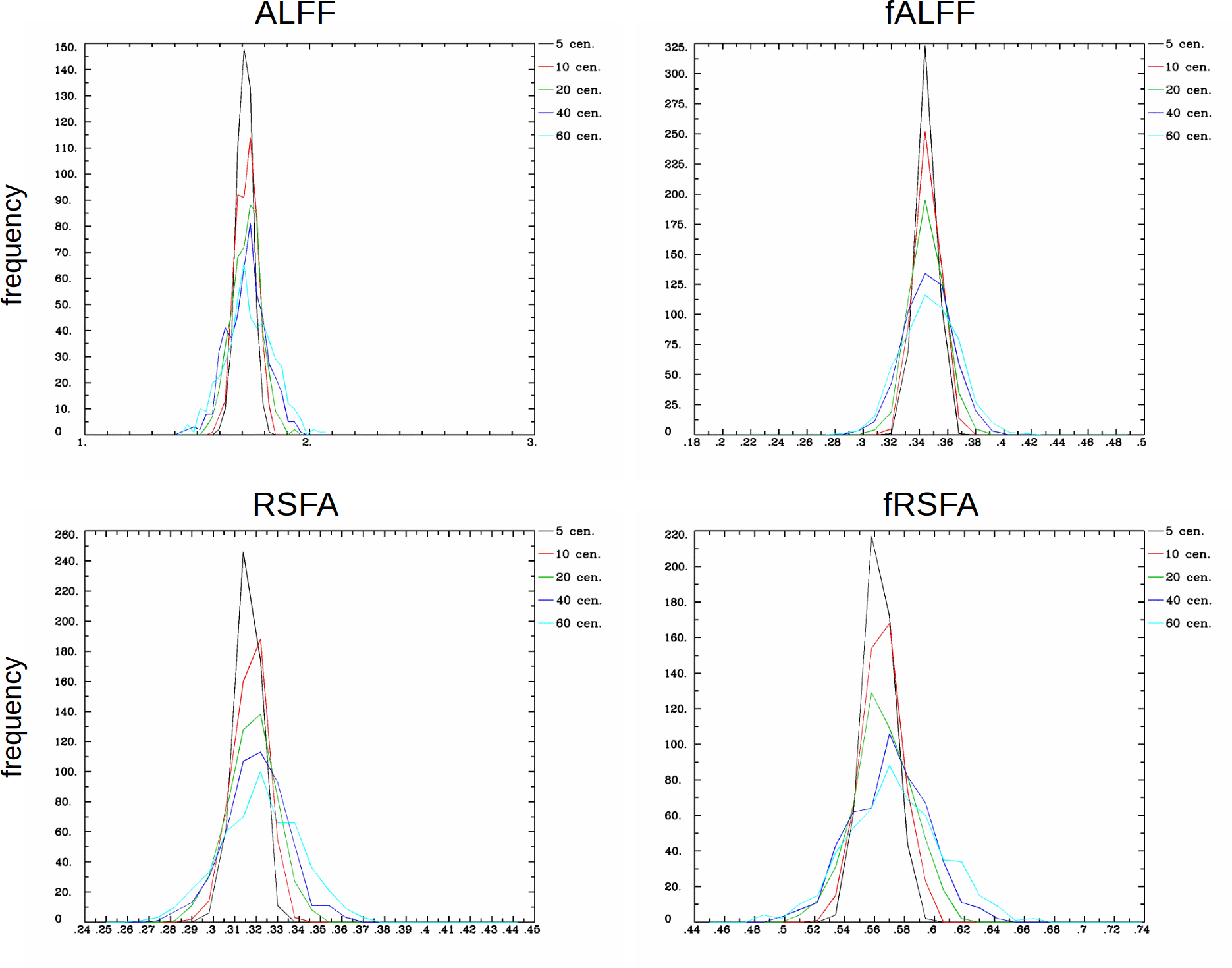
Distributions for each set and RSFC parameter are shown in Fig. 1. The distributions are unimodal and strongly peaked, peaked at approximately the same values. As expected, the distribution widens with increased censoring.

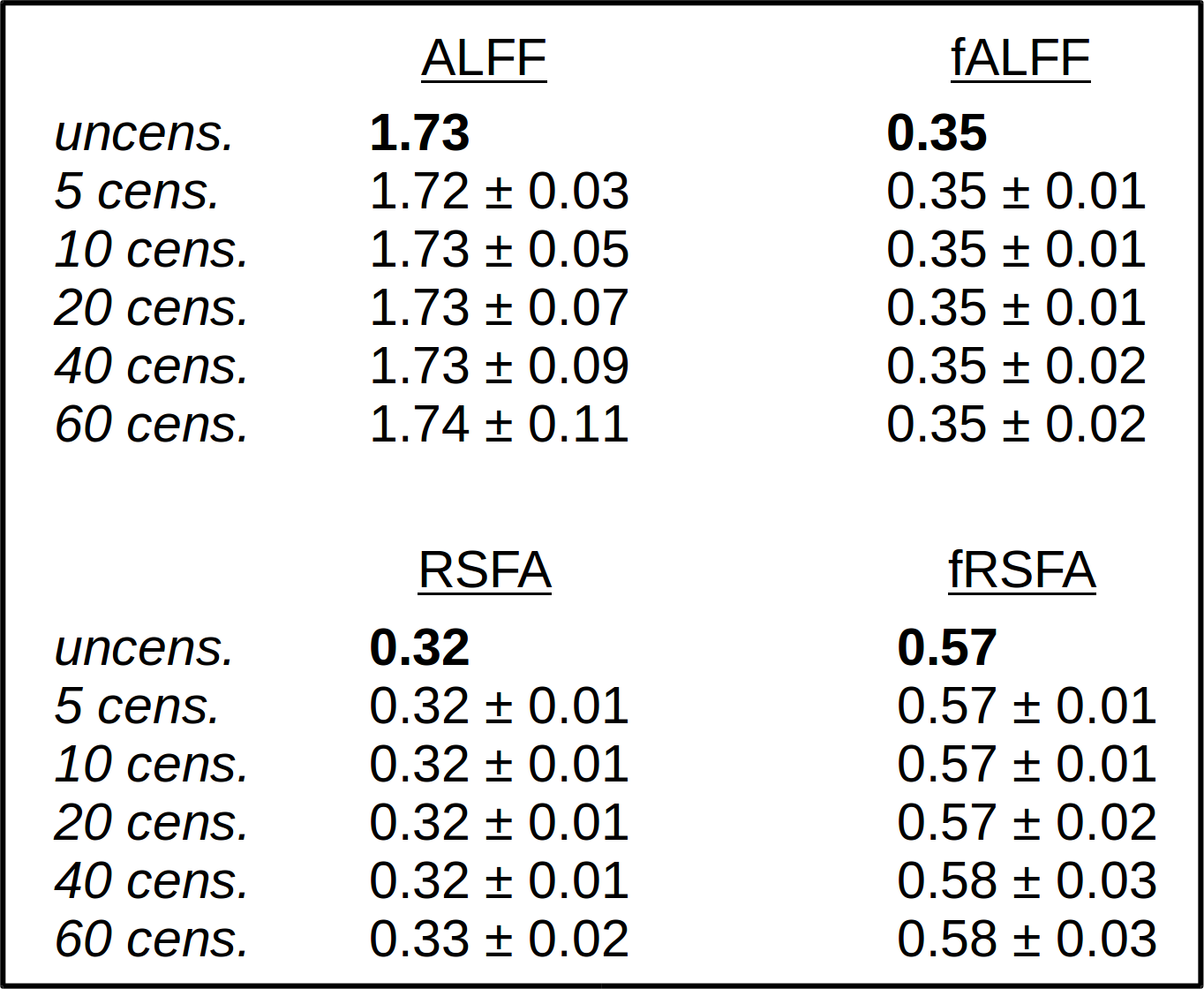
The mean and standard deviations for each level of censoring are shown in Fig. 2 for each RSFC parameter, along with the uncensored value for reference. Even at very high levels of censoring (up to nearly one third of the points), there does not appear to be significant bias in parameter estimate.

Conclusions

Acknowledgements

References

1. Zang YF, He Y, Zhu CZ, Cao QJ, Sui MQ, Liang M, Tian LX, Jiang TZ, Wang YF. 2007. Altered baseline brain activity in children with ADHD revealed by resting-state functional MRI. Brain Dev 29:83–91.

2. Zuo, X.N., Di Martino, A., Kelly, C., Shehzad, Z.E., Gee, D.G., Klein, D.F., Castellanos, F.X., Biswal, B.B., Milham, M.P., 2010. The oscillating brain: complex and reliable. Neuroimage 49:1432–1445.

3. Kannurpatti SS, Biswal BB. 2008. Detection and scaling of task induced fMRI-BOLD response using resting state fluctuations. Neuroimage 40:1567–1574.

4. Lomb, N. R. 1976, Ap&SS, 39, 447

5. Scargle, J. D. 1982, ApJ, 263, 835

6. Press, W. H., & Rybicki, G. B. 1989, ApJ, 338, 277

7. Eyer, L., & Bartholdi, P. 1999, A&AS, 135, 1

8. Taylor PA, Gohel S, Di X, Walter M, Biswal BB. 2012. Functional covariance networks: obtaining resting-state networks from intersubject variability. Brain Connect. 2(4):203-17.

9.

Cox RW. 1996. Comput Biomed Res 29:162-173.