Synopsis

DCE-MRI perfusion analysis suffers from low reliability, especially when 2^nd-generation pharmacokinetic models are used to estimate perfusion parameter maps (voxel-by-voxel estimation) in low SNR conditions. These models provide estimates of plasma flow and capillary permeability in addition to the commonly used parameters K^trans, k_ep. This contribution presents a method for estimation of perfusion maps using the tissue homogeneity model with incorporated spatial regularization in the form of total variation. The algorithm is based on the proximal minimization methods well established in image reconstruction problems. The use of state-of-the-art minimization and image regularization techniques stabilizes the estimates of perfusion parameter maps and keeps the computational demands low.

Introduction

Dynamic contrast-enhanced (DCE) MRI becomes an established tool to obtain information about tissue perfusion and vessel permeability. It is beneficial, when this information is represented by a set of physiological parameters (plasma flow, vascular volume, capillary permeability…) for each voxel in the region of interest, which gives so-called perfusion parameter maps. To get the parameter maps, the concentration-time curve of each voxel is fitted by a pharmacokinetic model. This curve-fitting is not trivial because of model nonlinearity, high dimensionality, insufficient temporal sampling and low signal-to-noise ratio (SNR), or uncertainties in either the model or measurement. This results in bias and uncertainty in the estimates or wrong estimates because of local minima¹.

A possible solution to overcome these problems is to use additional a priori information. Here, the nonlinear least squares curve-fitting problem is extended by a spatial regularization term (image prior) in the form of a total variation (TV), well known in image processing². This non-differentiable L₁-norm regularizer preserves piecewise smoothness of images. Other authors^1,3 have used differentiable spatial regularizers: Tikhonov, L_p norm for $$$p\in(1,2\rangle$$$, respectively, which tend to blur the solution. The main reason to use differentiable regularizers is to keep minimization tractable. We propose a method, which can handle state-of-the-art non-differentiable regularizers and reduces memory demands.

Method

The problem is formulated as a maximum a posteriori probability estimation, where the prior is in the form of a sum of 5 TV regularizations (sum of L₁ norms of the magnitude of image gradient). The data term is in the form of nonlinear least squares. The pharmacokinetic model is a time-domain convolution of a known arterial input function (AIF) with the tissue homogeneity model⁴ (TH). Its five parameters including bolus arrival time are to be estimated per each voxel. The convolution is evaluated in the Fourier domain because the TH model has no closed-form expression in the time domain.

The minimization is solved using the proximal gradient method⁵ to treat non-differentiability of the regularizer. The adopted algorithm iteratively repeats the following two steps until convergence: 1) perform one steepest descent step per each voxel, 2) evaluate the proximal operator to step 1). The evaluation of the proximal operator is in the form of the five image denoising problems, with different noise variances in each voxel, regularized by the used total variation. This sub-problem is solved by the Chambolle-Pock proximal algorithm⁶ adapted to the case with non-uniform noise variances. The sub-algorithm iteratively updates: 2a) per-voxel projection onto a unit circle in the domain of the image gradients, 2b) simple voxel-wise operations on the reconstructed image from 2a), 3b) voxel-wise update of perfusion map from 2b) using the solution from the previous iteration.

Evaluation and Discussion

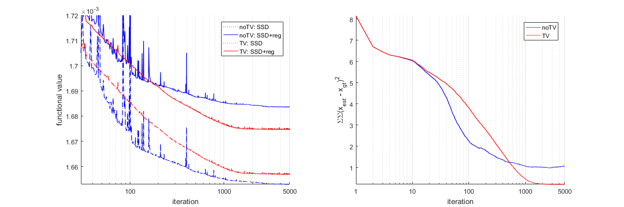
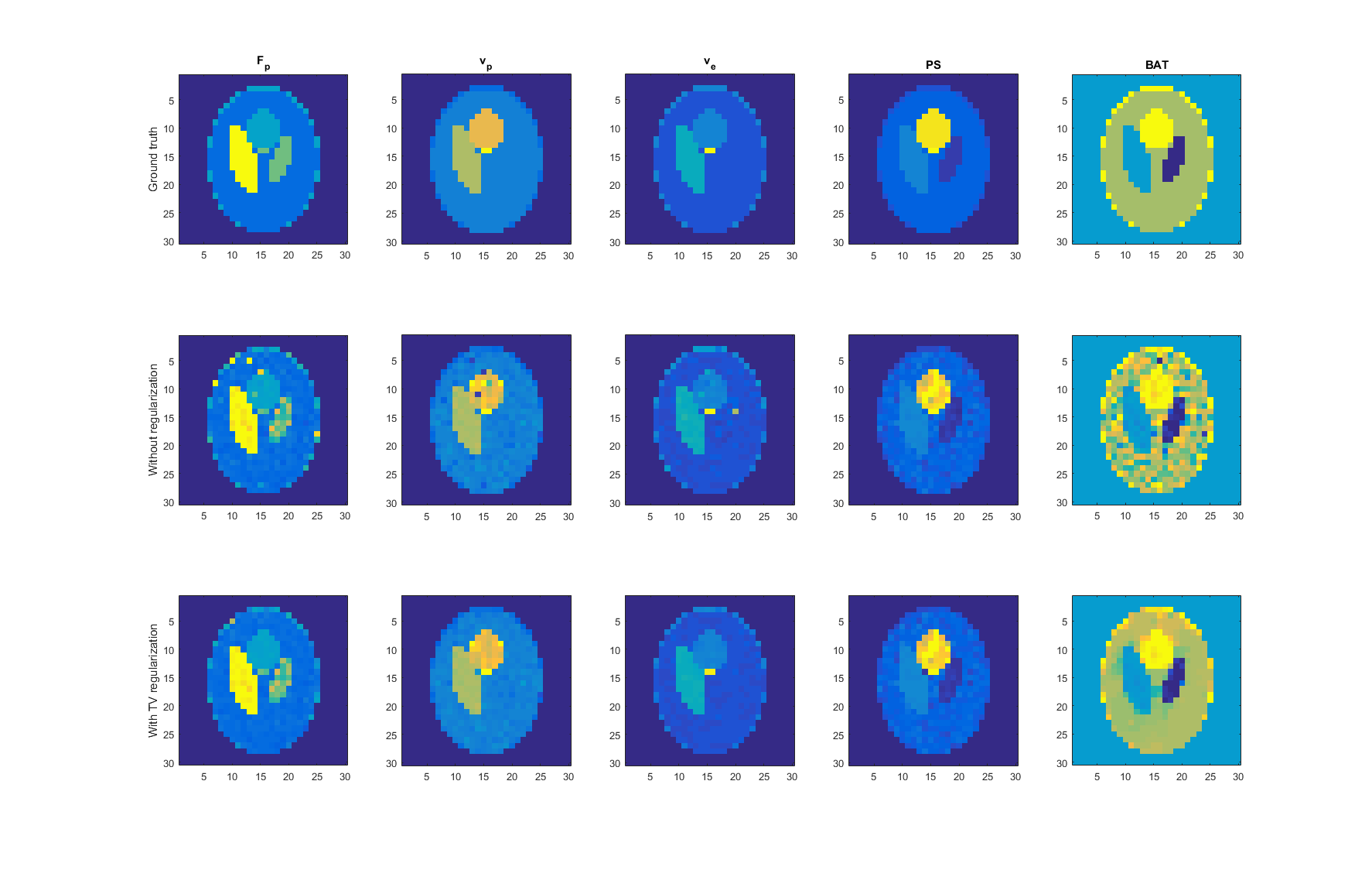
The algorithm was evaluated on simulated data based on the Shepp-Logan phantom and literature perfusion parameters and AIF (Figure 2 – top). The algorithm was qualitatively compared with its version with no TV regularization (Figure 2 – row 2, 3). The convergence properties (Figure 1) were also investigated. The regularization stabilized the estimation process (Figure 2 – column “BAT”) and reduced the number of outliers.

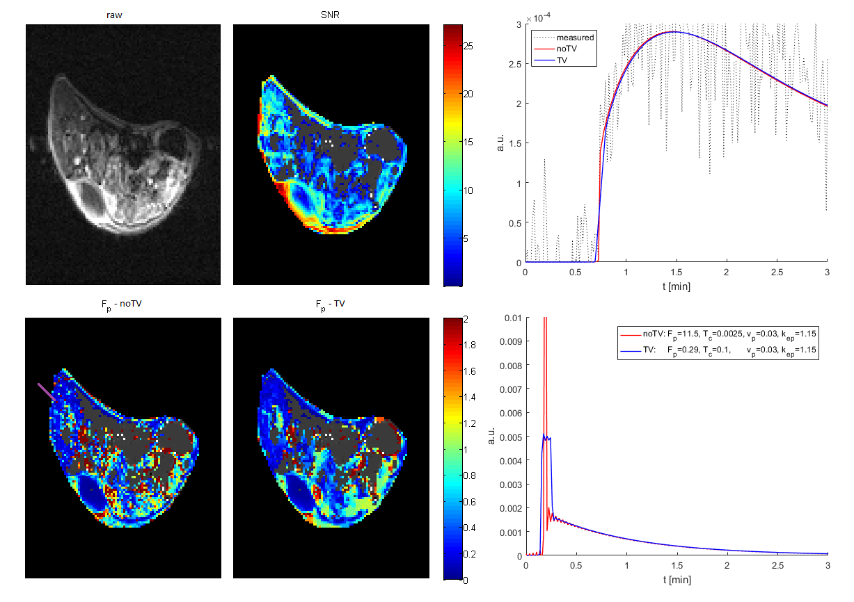
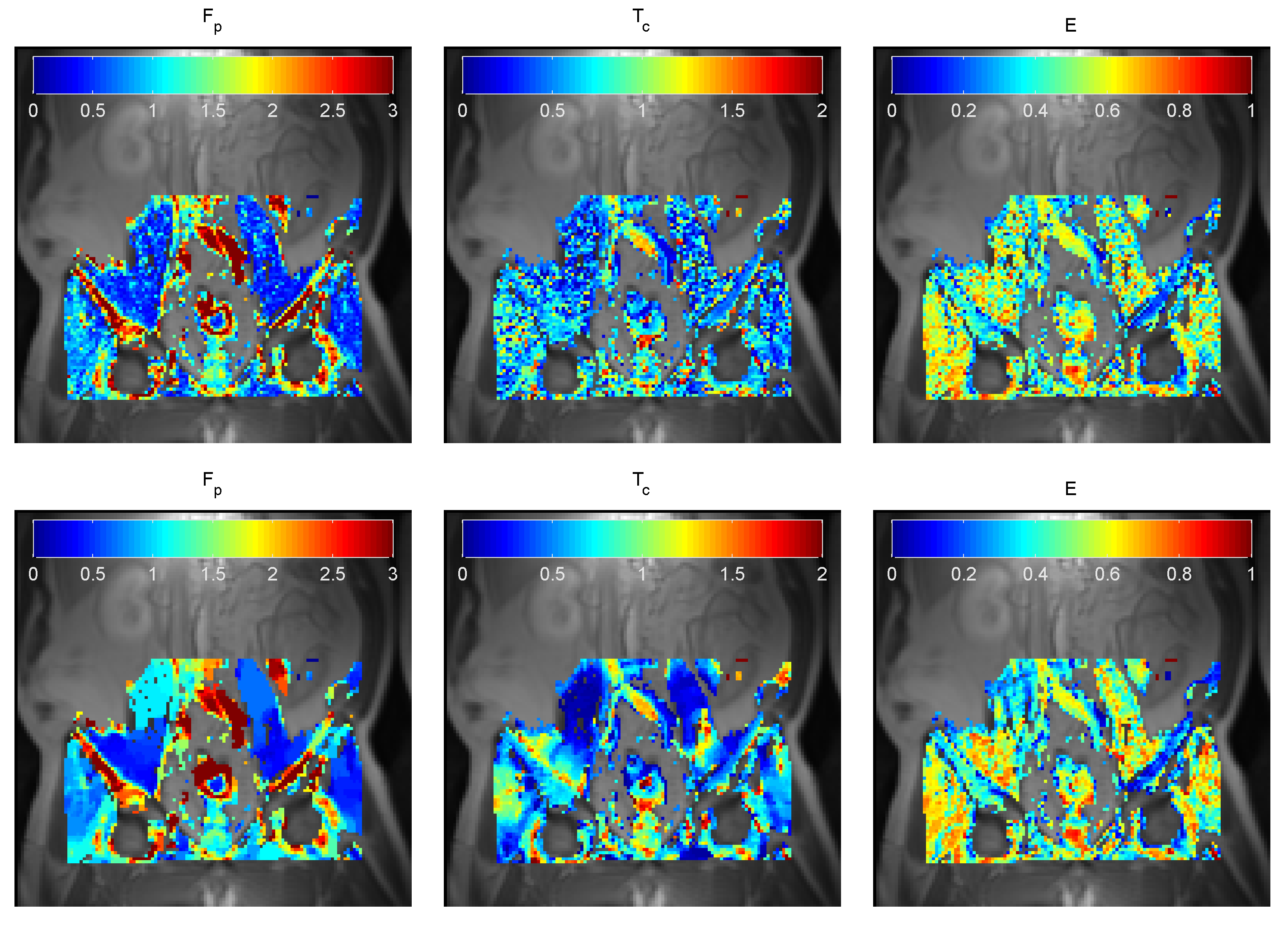
The potential of the algorithm to reduce outliers (no. of local minima) was also tested on a pre-clinical dataset (Figure 3) of BALB/C mice after subcutaneous implantation of tumor cells (CT26), approved by the National Animal Research Authority, and on an anonymized clinical dataset of a metastatic renal cell carcinoma in the pelvic area (Figure 4). In both cases, the readability of the estimated maps has increased, but the accuracy and precision, of the estimates need further investigation to be described quantitatively.

Conclusion

Acknowledgements

References

1. Kelm BM, Menze BH, Nix O, Zechmann CM, Hamprecht FA. Estimating Kinetic Parameter Maps From Dynamic Contrast-Enhanced MRI Using Spatial Prior Knowledge. IEEE Trans Med Imaging 2009;28:1534–47.

2. Rudin LI, Osher S, Fatemi E. Nonlinear total variation based noise removal algorithms. Phys D Nonlinear Phenom 1992;60:259–68.

3. Sommer JC, Gertheiss J, Schmid VJ. Spatially regularized estimation for the analysis of dynamic contrast-enhanced magnetic resonance imaging data. Stat Med 2014;33:1029–41.

4. Garpebring A, Ostlund N, Karlsson M. A Novel Estimation Method for Physiological Parameters in Dynamic Contrast-Enhanced MRI: Application of a Distributed Parameter Model Using Fourier-Domain Calculations. IEEE Trans Med Imaging 2009;28:1375–83.

5. Parikh N, Boyd S. Proximal Algorithms. Found Trends Optim 2013;1:123–231.

6. Chambolle A, Pock T. A first-order primal-dual algorithm for convex problems with applications to imaging. J Math Imaging Vis 2011;40:120–45.