2813

L1, Lp, L2, and Elastic Net Penalties for Regularization of Two-Gaussian Component Distributions in One-dimensional Magnetic Resonance Relaxometry

Christiana Sabett¹, Ariel Hafftka¹, Kyle Sexton², and Richard Spencer²

¹Applied Mathematics & Statistics, and Scientific Computation (AMSC), University of Maryland, College Park, College Park, MD, United States, ²National Institute on Aging (NIA), Baltimore, MD, United States

Synopsis

Magnetic resonance (MR) relaxometry time distributions are recovered via the inverse Laplace transform (ILT), an ill-posed problem that is generally stabilized using Tikhonov regularization. Recent work has considered other penalties, such as the L₁ penalty for locally narrow distributions. L_p penalties, 1<p<2, may be appropriate for distributions consisting of both narrow and broad components; a linear combination of L₁ and L₂ penalties, the elastic net (EN), may similarly be useful. However, there is little guidance regarding the choice of regularization penalty for the recovery of transverse relaxation distributions. We compare the effectiveness of each penalty for representative relaxation data.

PURPOSE

Magnetic resonance (MR) relaxometry is an emerging technique for characterizing biological tissues.^1-3Relaxation time distributions are recovered via the inverse Laplace transform (ILT), an ill-posed problem. This procedure is most often stabilized using Tikhonov regularization with an L₂ penalty, defined as the sum of the squared elements of the solution vector. Recent advances in computational methods and interest in sparsity have motivated additional work evaluating other penalties. The promotion of sparsity by the L₁ penalty is suitable for locally narrow transverse relaxation distributions.⁴ L_p penalties, 1<p<2, may be appropriate for distributions consisting of a combination of narrow and broad components; similarly, a linear combination of L₁ and L₂ penalties, the elastic net (EN), may be useful in such circumstances. However, there is little specific guidance regarding the choice of regularization penalty for the recovery of MR relaxation data. Here, we compare the effectiveness of each penalty for representative relaxation data.

THEORY

The discrete measured signal takes the form

$y(t_i)=\sum_{j=1}^KF(T_{2,j})e^{-t_i/T_{2,j}}$

where $y(t_i)$ denotes signal amplitude at acquisition times $t_i$ , typically integral multiples of an echo time (TE), $T_{2,j}$ denotes the decay time constant of the $j$ th component, and $F(T_{2,j})$ is its associated magnitude. In matrix form:

$y=AF$

where

$[A]_{i,j}=e^{-t_i/T_{2,j}},1\leq j\leq K$

is the $n\times K$ kernal, $y$ is the length- $n$ vector representing measurements at time points $t_i,1\leq i\leq n$ , and $F$ is a length- $K$ vector of amplitudes corresponding to possible relaxation times. With Tikhonov regularization, recovery of $F$ is cast as a nonnegatively constrained regularized least squares problem,

$\min_{F\geq0}\{||AF-y||_2^2+\alpha^2||F ||_2^2\}$

where $\alpha$ weights the regularization term relative to the fit residual. Similarly, for the L₁ penalty, we have

$\min_{F\geq0}\{||AF-y||_2^2+\alpha||F ||_1\}$

while the L_p penalty appears as

$\min_{F\geq0}\{||AF-y||_2^2+\alpha||F ||_p\}$

and the EN penalty as

$\min_{F\geq0}\{||AF-y||_2^2+\alpha_1||F ||_1+\alpha_2||F ||_2\}$

METHODS

Our input model consists of a bimodal T₂ distribution with Gaussian peaks, each characterized by mean T₂ and standard deviation (SD). For L_p penalties, the regularization parameter was established within a range of [10^-7,10^-1]. For the EN penalty, a 5×5 grid search was performed across a range of [10^-6,10^-2] for α₁ and a range of [10^-7,10^-3] for α₂. Minimizations were performed using CVX software.⁵ The unknown model vector

$F$ consisted of 176 allowable T₂ rates, logarithmically spaced between 10 and 1000 ms. Noise-free decay data was generated at 352 discrete TE values, and then corrupted with additive white Gaussian noise, appropriate for spectroscopic or high signal-to-noise imaging experiments. Performance was evaluated using mean-squared error between the input model and the recovered distribution, normalized by the sum of the squared values of the input model.

RESULTS

Figure 1 demonstrates the superiority of the L₁ penalty in recovering a narrow distribution (Fig. 1a), and the superiority of the L₂ penalty in recovering a wider-peak distribution (Fig. 1b). The heat maps in Figure 2a and 2b show performance across a range of models with varying (but equal in each peak) linewidths, and varying separations, for the L₂ and L₁ penalties, respectively. The L₂ penalty is seen to perform well overall, but poorly for overlapping peaks. The L₁ penalty clearly begins to fail as peak width increases, as expected. Figure 3 defines the optimal penalty across the same range of linewidths and peak separations. For a distribution of peaks of unequal SD, Figure 4 shows better performance by the L_1.5 penalty as compared to the L₂ penalty. Finally, Figure 5 demonstrates T₂ distribution recovery for normal and osteoarthritic human cartilage samples,¹ showing that all penalties recovered a bimodal distribution with roughly consistent peak centers but with markedly different peak SD. Based on our simulation analysis, we expect that the L_1.5 recovery is likely to be the most appropriate.

DISCUSSION

For sparse distributions, we find that the L₁ penalty is optimal. The L₂ penalty performs very well across a wide range of parameter values, underscoring the robustness of conventional Tikhonov regularization. Of particular interest are distributions with unequal peak widths, where neither the emphasis on sparsity from the L₁ penalty nor the emphasis on smoothness in the L₂ penalty are fully optimal. We found that the L_1.5 and EN penalties were more successful in modeling this situation. Of these the elastic net promotes sparsity, but requires optimization over two regularization parameters, so that the L_1.5 may be preferred overall. Overall, our results demonstrate the regions where the use of a particular regularization penalty term is likely to be most appropriate, and can be implemented in the usual case in which the experimentalist has a priori knowledge of the general characteristics of an underlying model distribution.

Acknowledgements

This work was supported by the Intramural Research Program of the NIH, National Institute on Aging. We thank John Benedetto and Alfredo Nava-Tudela of the University of Maryland for their interest and comments. Tissue samples were kindly provided by Dr. Tariq A. Nayfeh.

References

Reiter DA, Irrechukwu O, Lin P-C, Moghadam S, Thaer SV, Pleshko N, et al. Improved MR-based characterization of engineered cartilage using multiexponential T2 relaxation and multivariate analysis. NMR in Biomedicine. 2012;25(3):476-88.
Reiter DA, Roque RA, Lin P-C, Irrechukwu O, Doty S, Longo DL, et al. Mapping proteoglycan-bound water in cartilage: Improved specificity of matrix assessment using multiexponential transverse relaxation analysis. Magnetic Resonance in Medicine. 2010;65(2):377-84.
Reiter DA, Lin P-C, Fishbein KW, Spencer RG. Multicomponent T2 relaxation analysis in cartilage. Magnetic Resonance in Medicine. 2009;61(4):803-9.
Berman P, Levi O, Parmet Y, Saunders M, Wiesman Z. Laplace Inversion of Low-Resolution NMR Relaxometry Data Using Sparse Representation Methods. Concepts in Magnetic Resonance Part A. 2013;42A(3):72-88.
Grant M, Boyd S. CVX: Matlab software for disciplined convex programming. 2.0 beta ed2013.

Figures

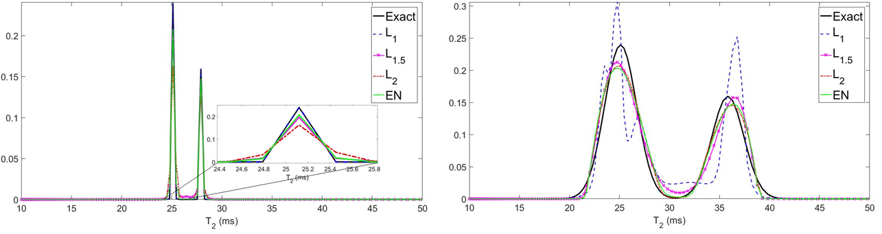
Figure 1a. (Left) Comparison of methods for recovery of two noiseless, closely-spaced, narrow Gaussian peaks, centered at 25 ms and 27.8 ms, with equal standard deviations of 0.1 ms. Note the superiority of the EN penalty over the L₂ but not the L₁ penalty, and similar performance of the L_1.5 and EN penalties.

Figure 1b. (Right) Comparison of methods for recovery of two noiseless Gaussian peaks, wider than those of Figure 1a, centered at 25 ms and 35.9 ms, with equal standard deviations of 1.6 ms. Note the failure of the L₁ penalty, and similar performance of the other penalties.

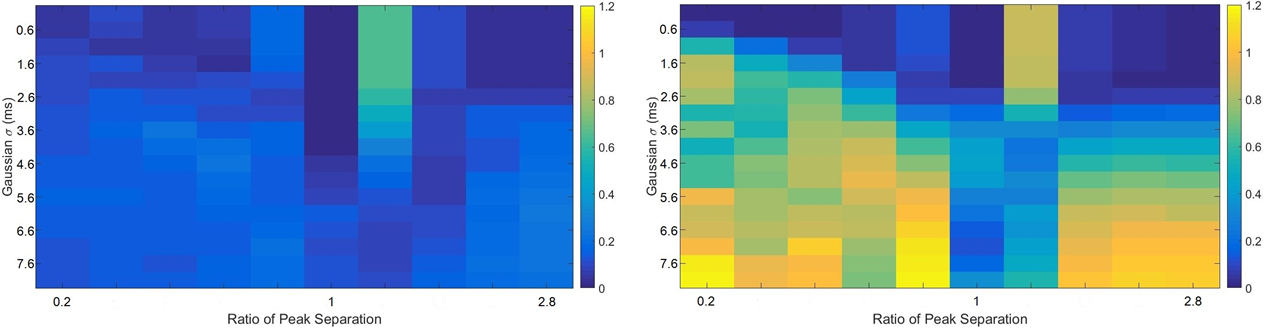
Figure 2. Average relative error over 20 trials, SNR 700, corresponding to peak width and peak separation for two Gaussian peaks of equal SD. The top leftmost square in the grids represents the relative error for the distribution with the most closely spaced and narrowest peaks. Moving right along the grids corresponds to changing the distance between the peaks, expressed as a ratio of peak centers along the T₂ axis.

a. (Left) L₂ penalty error. Note the general consistency of the recovery, best for well-separated, non-overlapping peaks.

b. (Right) L₁ penalty error. Note the decrease in good recovery as peak width increases.

Figure 3. Ratio of average relative errors of L₂/L₁ penalties across 20 trials corresponding to peak width and peak separation for two Gaussian peaks of equal SD. The green lines delimit the regions for which the two penalties recover distributions with errors within 15% of each other. The red lines delimit regions for which the L₁ penalty outperforms the L₂ penalty by > 15% in mean square error. Note the preference for the L₁ penalty for narrow-peak distributions, and the shift to better performance by the L₂ penalty in the case of distributions with wider peaks.

Figure 4. Comparison of methods in recovering a distribution of Gaussian peaks, centered at 25 ms and 59.9 ms, with SD of 1.6 ms and 8 ms, respectively. Note the increased fidelity of the L_1.5 penalty as compared to the L₂ penalty, and the overall failure of the L₁ penalty.

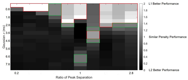
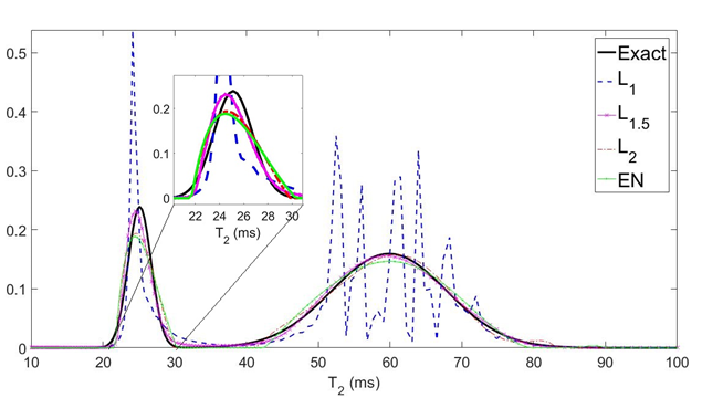
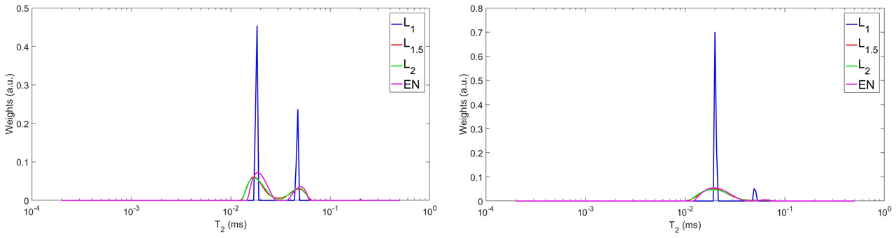
Figure 5. Magnetic resonance transverse relaxation time (T₂) data for human cartilage explants taken from the tibial plateau.

a. (Left) This sample was obtained from an arthroplasty procedure and represents visually non-degraded tissue. Note the consistency of identified peak centers across all penalty terms.

b. (Right) This sample was obtained from the same arthroplasty procedure as in Fig. 5a, and represents visually degraded tissue. Comparing Fig. 5b with 5a, it is seen that the degraded tissue exhibits a larger average T₂ value and a broader distribution as compared to the non-degraded sample. This indicates the extent of tissue breakdown within the osteoarthritic cartilage.

Proc. Intl. Soc. Mag. Reson. Med. 26 (2018)

2813