2801
AUTOMAP Image Reconstruction of Low Signal-to-Noise MR Data at 6.5 mT1Radiology, Athinoula A. Martinos Center for Biomedical Imaging, Massachusetts General Hospital, Charlestown, MA, United States, 2Harvard Medical School, Boston, MA, United States, 3Physics, Harvard University, Cambridge, MA, United States
Synopsis
Due to very low Boltzmann polarization, MR images acquired at ultra-low field (ULF), MR images are mostly corrupted with noise, thus resulting in low signal-to-noise. In the aim of improving image quality at ULF, we apply the deep neural network image reconstruction technique, AUTOMAP, to low SNR datasets acquired at 6.5 mT. The performance of AUTOMAP (Automated Transform by Manifold Approximation) versus the conventional Inverse Fast Fourier Transform (IFFT) on this data was evaluated. The results for AUTOMAP reconstruction show a significant noise reduction, leading to more than 30% gain in signal to noise ratio as compared to standard IFFT.
Introduction
MR Imaging at ultra low field (ULF) suffers from low signal-to-noise ratio (SNR) due to intrinsically low Boltzman polarization. As a result, long acquisition times are needed to accommodate the additional signal averaging required to attain sufficient SNR. We recently developed a noise-robust image reconstruction approach based on a data-driven learning of the low-dimensional manifold representations of real-world data, and implemented with a deep neural network architecture. AUTOMAP – Automated Transform by Manifold Approximation1 – is an end-to-end automated k-space-to-image-space generalized reconstruction framework that learns a highly-parameterized image reconstruction function optimized for a corpus of training data, and is less sensitive to input corruptions such as channel noise. Here, we assessed the performance of AUTOMAP on ULF MR data acquired at 6.5 mT, and compared the results with those obtained with the conventional Inverse Fast Fourier Transform (IFFT) reconstruction method.Materials and Methods
Training set: The training corpus was assembled from 50,000 2D T1-weighted brain MR images selected from the MGH-USC Human Connectome Project (HCP)2 public database. The images were cropped to 256 × 256 and were subsampled to 64 × 64, symmetrically tiled to create translational invariance and finally normalized to the maximum intensity of the data. To produce the corresponding k-space representations for training, each image was Fourier Transformed with MATLAB’s native 2D FFT function.
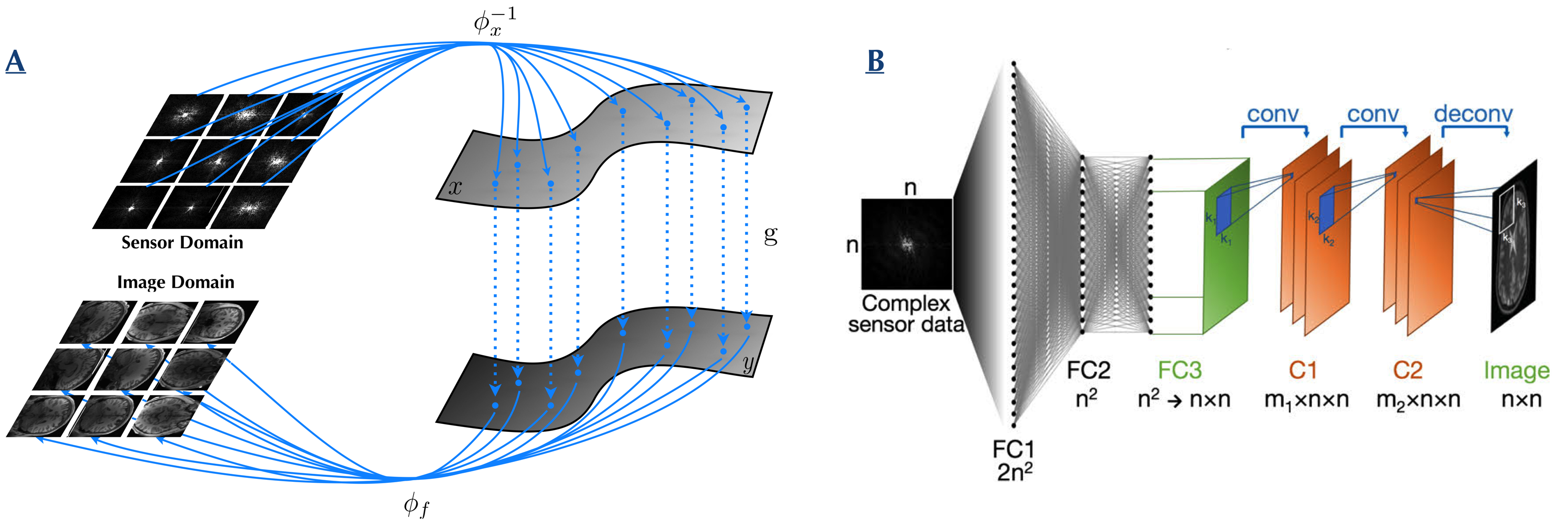
Architecture of NN: The NN was trained to learn an optimal feed-forward reconstruction of k-space domain into the image domain. The real and the imaginary part of datasets were trained separately. The network, described in Figure 1, was composed of 3 fully connected layers (input layer and 2 hidden layers) of dimension n2 × 1 and activated by the hyperbolic tangent function. The 3rd layer was reshaped to n × n for convolutional processing. Two convolutional layers convolved 128 filters of 3 × 3 with stride 1 followed each by a rectifier nonlinearity. The last convolution layer was finally de-convolved into the output layer with 64 filters of 5 × 5 with stride 1. The output layer resulted into either the reconstructed real or imaginary component of the image. The details of the training parameters used for this study are described in Ref 1.
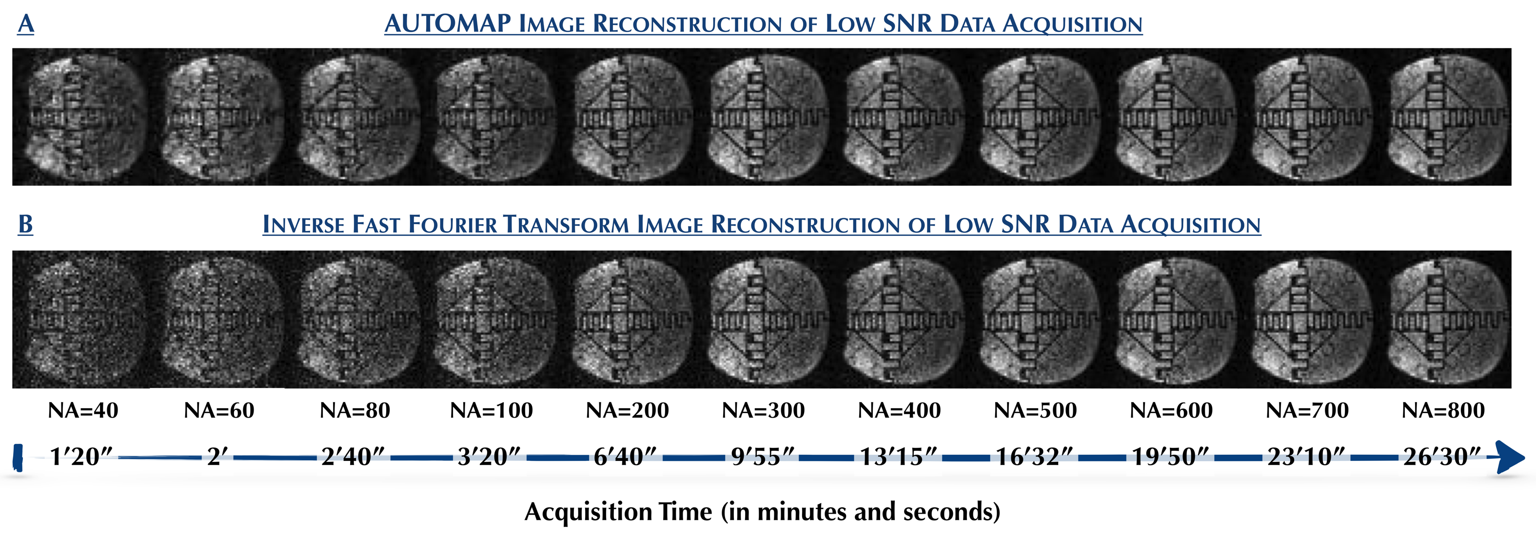
Data Acquisition: 2D ULF data at 6.5 mT were acquired with a balanced Steady State Free Precession (b-SSFP) 3 sequence using a hemispheric water-filled structured resolution phantom placed inside a single-channel spiral volume head coil4. The sequence parameters were: TR =31ms, matrix size = 64 × 64, spatial resolution = 4.2 mm × 3.6 mm, and a slice thickness = 12 mm. The number of averages (NA) were set to 40, 60, 80, 100, 200, 300, 400, 500, 600, 700, and 800 respectively. The total acquisition time of each dataset is shown in Figure 2.
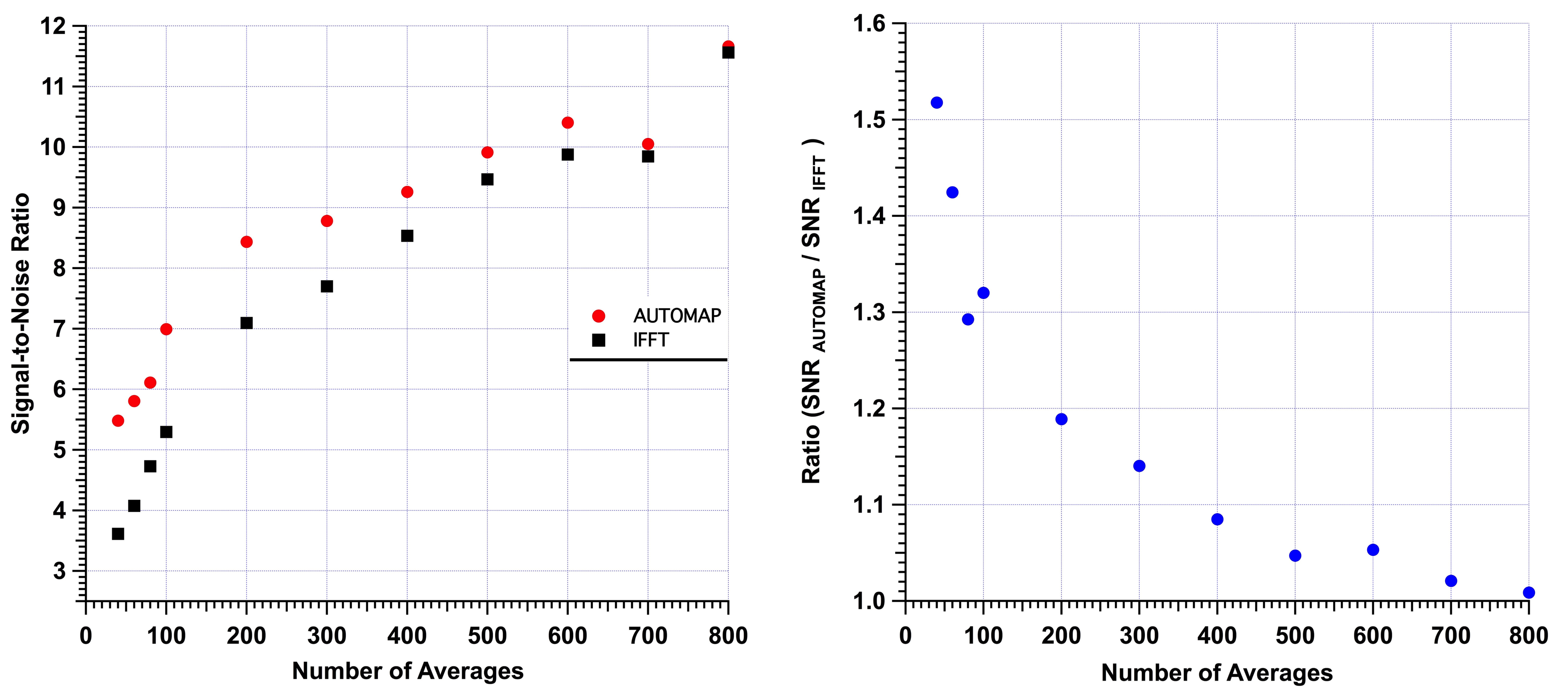
Data Analysis: The signal magnitude of each dataset was normalized to unity to enable fair comparison between both reconstruction methods. SNR was then computed by dividing the signal magnitude by the standard deviation of the noise. The gain in SNR was also calculated by taking the ratios of SNRs of the AUTOMAP reconstructed images over the IFFT reconstructed images.
Results
Figure 2 shows 2D b-SSFP images acquired with increasing NA, reconstructed by either AUTOMAP (upper panel) or by the conventional FFT (lower panel) reconstruction methods. Significantly noise-reduced images were obtained, particularly at lower N, with the AUTOMAP reconstruction method. At very low SNR, more detailed structures of the phantom were identifiable with AUTOMAP. SNR calculations (in Figure 3a) show the performance of AUTOMAP with a higher SNR (red line) than IFFT reconstructed images (black line); the gain in SNR for a 3-minute 2D scan with 100 averages was ~ 30% (in Figure 3b). This increase in SNR is equivalent to the IFFT reconstruction of a 200-average 7-minute scan time. Hence, AUTOMAP enables a significant reduction in scan time of nearly 2-fold for very low NA.Discussion & Conclusion
The reconstruction performance of AUTOMAP on low SNR data demonstrates the robustness of the reconstruction technique and its high immunity to noise in the ULF regime. The significant noise reduction will enable substantial scan time reduction at ULF. Application of AUTOMAP to 3D acquisitions is also currently in progress, where we anticipate even greater noise robustness potential as the low-dimensional features present in the third dimension due to smoothly-varying anatomical continuity will further constrain the reconstruction problem.Acknowledgements
No acknowledgement found.References
1.‘Image reconstruction by domain transform manifold learning’, B. Zhu and J. Z. Liu and B. R. Rosen and M. S. Rosen, arXiv:1704.08841, (2017).
2. ‘MGH–USC Human Connectome Project datasets with ultra-high b-value diffusion MRI’, Fan, Q. et al. NeuroImage 124, 1108–1114 (2016).
3. ‘Low-Cost High-Performance MRI’, M. Sarracanie, C. D. LaPierre, N. Salameh, D. E. J. Waddington, T. Witzel and M. S. Rosen, Scientific Reports 5 15177 (2015)
4. ‘A single channel spiral volume coil for in vivo imaging of the whole human brain at 6.5 mT’, C. D. LaPierre , M. Sarracanie, D. E. J. Waddington and M. S. Rosen, ISMRM abstract Proc. Intl. Soc. Mag. Reson. Med. 23 (2015) 5902
Figures