2791
Deep Learning for Magnetic Resonance Fingerprinting: Accelerating the Reconstruction of Quantitative Relaxation Maps1Pattern Recognition Lab, Department of Computer Science, Friedrich-Alexander-Universität Erlangen-Nürnberg, Erlangen, Germany, 2Siemens Healthcare, Application Development, Erlangen, Germany, 3Friedrich-Alexander-Universität Erlangen-Nürnberg, Erlangen, Germany
Synopsis
This work demonstrates the successful application of Deep Learning with phantom and human measurements for the reconstruction in Magnetic Resonance Fingerprinting (MRF). State-of-the-art MRF reconstruction yields quantitative maps of e.g. T1 and T2 by acquiring multiple undersampled images with various acquisition parameters, commonly referred to as fingerprints. Every measured fingerprint (per voxel) is compared with a dictionary of simulated fingerprints for possible parameter combinations. This time-consuming step can be replaced with a neural network, which directly predicts the parameters from a fingerprint. This was previously shown with simulated data. Here, we extend this approach to real measurements.
Introduction
In Magnetic Resonance Fingerprinting (MRF), many strongly undersampled images with various acquisition parameters like flip angle (FA) or repetition time (TR) are recorded in order to generate a so-called fingerprint per voxel (Figure 1A), from which quantitative maps of e.g. T1 and T2 relaxations can be computed.1,2 The state-of-the-art reconstruction is time-consuming, since it compares every fingerprint to a dictionary of simulated fingerprints of possible parameter combinations to retrieve the best matching entry.1,2 Deep Learning (DL) can be used to reformulate the MRF reconstruction as a regression task with the help of neural networks. Previous approaches used either fully-connected neural networks3,4 or Convolutional Neural Networks (CNNs).5 The first method utilized a 25-point MRF EPI6 pulse sequence, which did not lead to undersampling artifacts such as ours (Figures 1A+B). The second approach showed the applicability of a CNN similar to our prototype sequence with simulated data.5 In this work, we extend the second approach,5 which directly predicts quantitative parameters from fingerprints. We train a CNN on measured (phantom and human) fingerprints and show as a proof-of-concept that it offers accurate and faster reconstruction despite the severly undersampled acquisition.Methods
2D MRF data was acquired using Fast Imaging with Steady
State Precession2 on a MAGNETOM Skyra 3T (Siemens Healthcare,
Erlangen, Germany) with a prototype sequence with the following parameters:
Field-of-View 300×300 mm2
For the network architecture, convolutional layers in addition to fully-connected layers were used because the fingerprint is expected to be correlated along the time dimension. Previous training with simulations5 was a much easier task since no undersampling artifacts were considered. We now extend the previous CNN architecture5 to be able to cope with these strong undersampling effects (factor 48) and train it on our measured data. The architecture of our CNN for the phantom (human) data consists of 4 (6) convolutional layers, average pooling and 4 (6) fully-connected layers with Rectified Linear Units8 as activation functions (Figure 2). Data from 20 (6) phantom (human) measurements with 21,940 (110,670) signals (Figure 1C+D) was used, separated randomly for training (90%) and validation (10%). We implemented our method using the TensorFlow library.9 The weights were initialized randomly.10 For optimization we used the ADAM method11 (initial learning rate: 5·10-4) and minimized the mean squared error as a loss function.
Results
Testing was performed on a set of two independent phantom and human measurements. Results show a small error compared to the ground truth MRF reconstruction1,2 (mean error±standard deviation, phantom (human): T1: 11.3±11.5 ms (92±167 ms), T2: 3.4±4.3 ms (19±44 ms), Figures 3+4). Deeper architectures lead to better accuracy with measured fingerprints (Figure 5).
Execution time was
compared on a 2.7 GHz Intel Core i5: While the state-of-the-art reconstruction1,2 requires approximately 61 ms for one
fingerprint with a dictionary of 10,098 T1 and T2 combinations, the CNN method can improve this
by a factor of 10 (7) for phantom (human) data on the same hardware. We can
further accelerate this by a factor of ≈
Discussion
Figures 1A+B show the substantially increased difficulty for a MRF reconstruction caused by the undersampling artifacts arising from the accelerated acquisition scheme and other artifacts for human data due to the living object of investigation compared to simulated fingerprints. We showed that our proposed CNNs can cope with this added difficulty. This is possible due to the deeper architectures of our networks compared to the previous one for simulated data.5 In comparison to the previously proposed DL approach without undersampling artifacts and with a coarser image resolution (2×2 mm2, 128×128 matrix),3,4 our images (1.17×1.17 mm2, 256×256 matrix) are clinically more relevant ones.Conclusion
The CNN-based reconstruction has been shown to be applicable to real measured fingerprints of MRF acquisitions with strong undersampling and to yield accurate predictions of quantitative parameter maps. It further provides the advantages of reduced computational effort and predicted continuous values instead of limited discrete parameters contained in the dictionary. Further work will focus on architectural and image quality improvements for human data.Acknowledgements
No acknowledgement found.References
1. Ma D, Gulani V, Seiberlich N, et al. Magnetic resonance fingerprinting. Nature. 2013; 495(7440):187-92. doi: 10.1038/nature11971.
2. Jiang Y, Ma D, Seiberlich N, et al. MR fingerprinting using fast imaging with steady state precession (FISP) with spiral readout. Magnetic Resonance in Medicine. 2015;74(6):1621-31. doi: 10.1002/mrm.25559.
3. Cohen O, Zhu B, Rosen MS. Deep learning for fast MR fingerprinting reconstruction. In: Proceedings of the International Society for Magnetic Resonance in Medicine. Honolulu, HI, USA; 2017. p. 688.
4. Cohen O, Zhu B, Rosen MS. Deep Learning for Rapid Sparse MR Fingerprinting Reconstruction. arXiv preprint, arXiv:1710.05267, 2017.
5. Hoppe E, Körzdörfer G, Würfl T, et al. Deep Learning for Magnetic Resonance Fingerprinting: A New Approach for Predicting Quantitative Parameter Values from Time Series. Studies in health technology and informatics. 2017;202-6.doi: 10.3233/978-1-61499-808-2-202.
6. Cohen O, Sarracanie M, Armstrong BD, et al. Magnetic resonance fingerprinting trajectory optimization. In: Proceedings of the International Society for Magnetic Resonance in Medicine; Milan, Italy; 2014. p. 27.
7. High Precision Devices, Inc. Calibrate MRI Scanners with NIST Referenced Quantitative MRI (qMRI) Phantoms (QIBA DWI and ISMRM). http://www.hpd-online.com/MRI-phantoms.php. Accessed October 16, 2017.
8. Glorot X, Bordes A, Bengio Y. Deep sparse rectifier neural networks. In: Proceedings of the Fourteenth International Conference on Artificial Intelligence and Statistics. Ft. Lauderdale, FL, USA; 2011. p. 315-23.
9. Abadi M, Agarwal A, Barham P, et al. Tensorflow: Large-scale machine learning on heterogeneous distributed systems. arXiv preprint, arXiv:1603.04467, 2016.
10. Glorot X, Bengio Y. Understanding the difficulty of training deep feedforward neural networks. In: Proceedings of the Thirteenth International Conference on Artificial Intelligence and Statistics. Sardinia, Italy; 2010. p. 249–56.
11. Kingma D, Ba, J. Adam: A method for stochastic optimization. arXiv preprint arXiv:1412.6980, 2014.
Figures
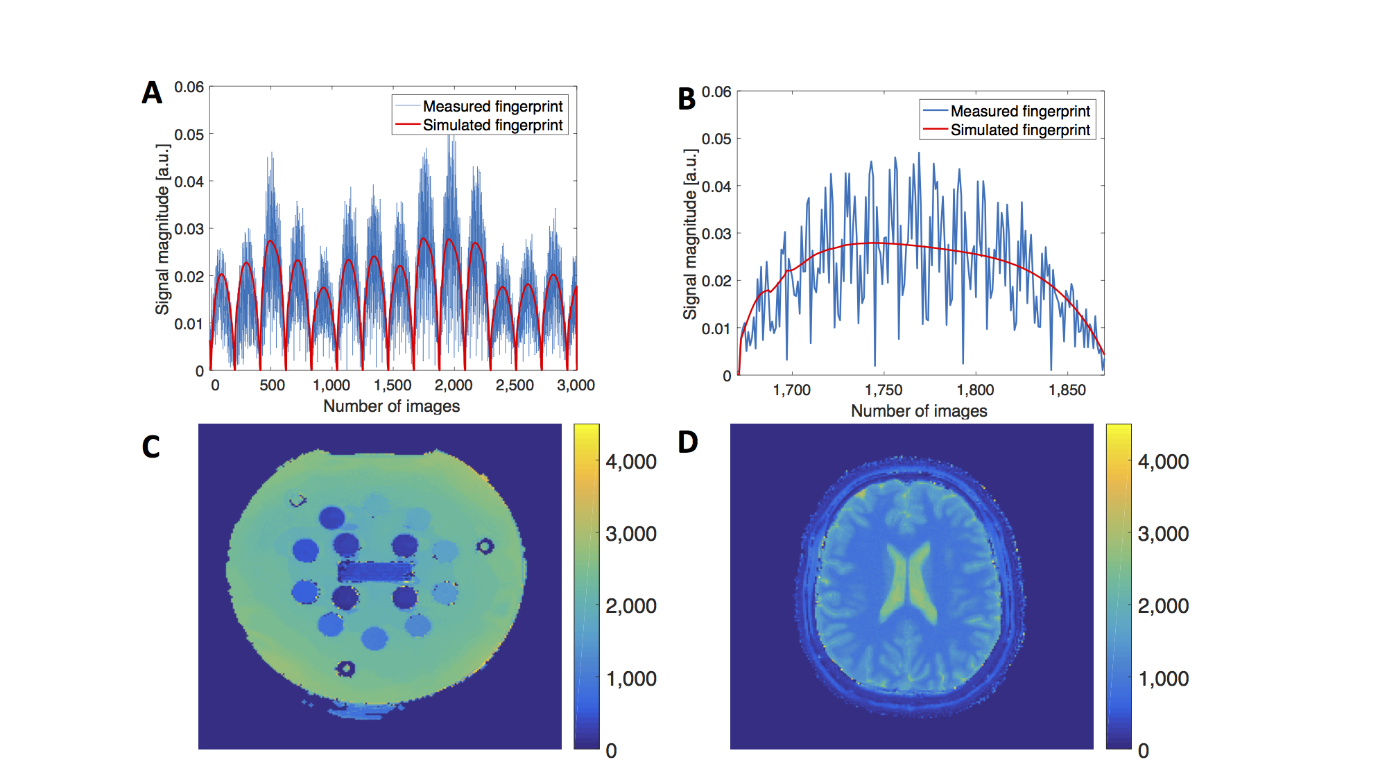
Figure 1: Fingerprints from the used acquisition scheme and reconstructed quantitative maps with the state-of-the-art MRF method1,2
A+B: Exemplary measured fingerprint from a ISMRM/NIST phantom (blue) and the associated simulated fingerprint from the dictionary (red, parameters: T1: 240 ms, T2: 160 ms). A: Whole signal (3,000 data points), B: Enlarged excerpt from A to clarify the differences between simulated and measured fingerprints.
C+D: Example of quantitative relaxation maps of one ISMRM/NIST (C) and one human (D) measurement. Both T1 maps, in units of ms.
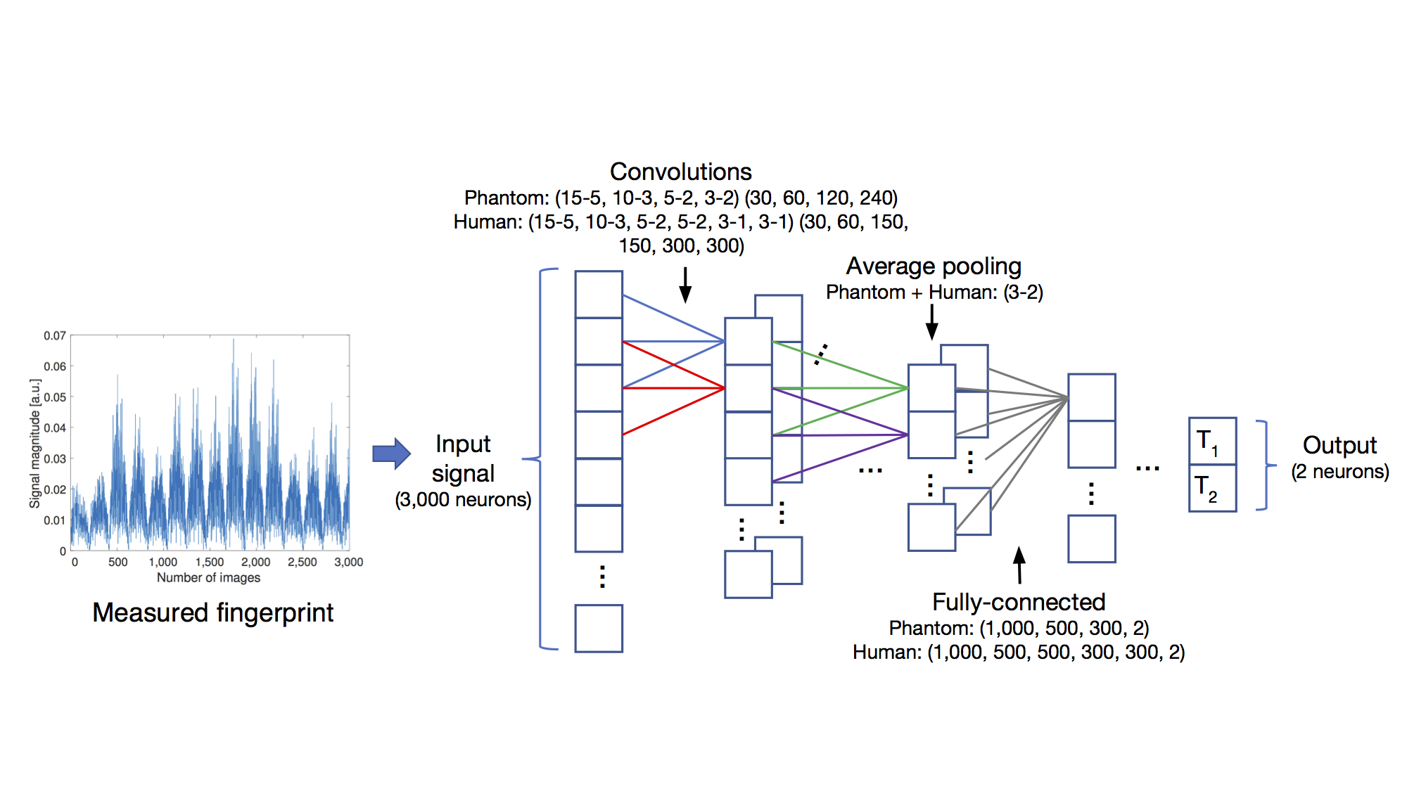
Figure 2: Schema of our proposed CNNs, which directly predict quantitative parameters from a fingerprint, instead of comparing it to a dictionary consisting of simulated fingerprints for every parameter combination. The input layer consists of 3,000 neurons for the 3,000 data points from the measured fingerprint (phantom or human), followed by 4 (phantom data) or 6 (human data) convolutional layers (given in the following form: (kernel size-stride size per layer) (feature maps per layer) ), average pooling (kernel size-stride size) and 4 (phantom data) or 6 (human data) fully-connected layers (number of neurons per layer).
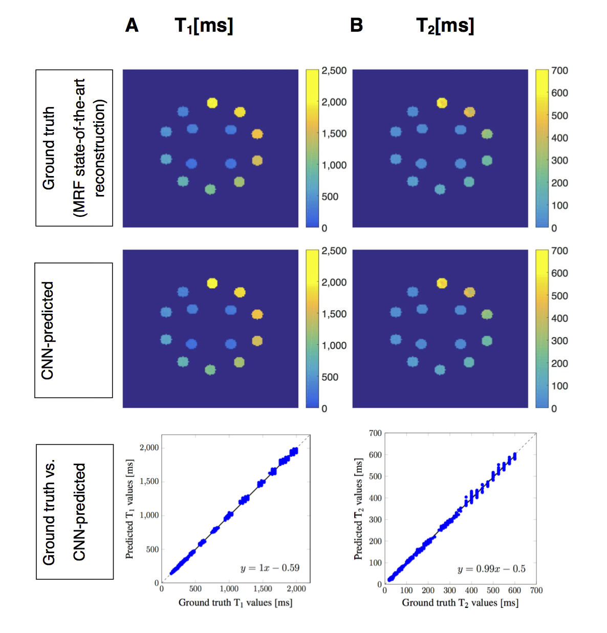
Figure 3: Prediction results from the proposed CNN in Figure 2 for phantom data. A: T1, B: T2. First row: Ground truth (state-of-the-art MRF reconstruction) quantitative relaxation maps (masked balls) in units of ms. Second row: CNN-predicted quantitative relaxation maps (masked balls) in units of ms. Third row: Ground truth versus predicted values. The dashed line is the x=y line, the solid line is the linear regression (with its formula in the right corners). The results show, that our CNN was able to predict accurate quantitative values from measured phantom fingerprints and yielded small errors compared to the ground truth.
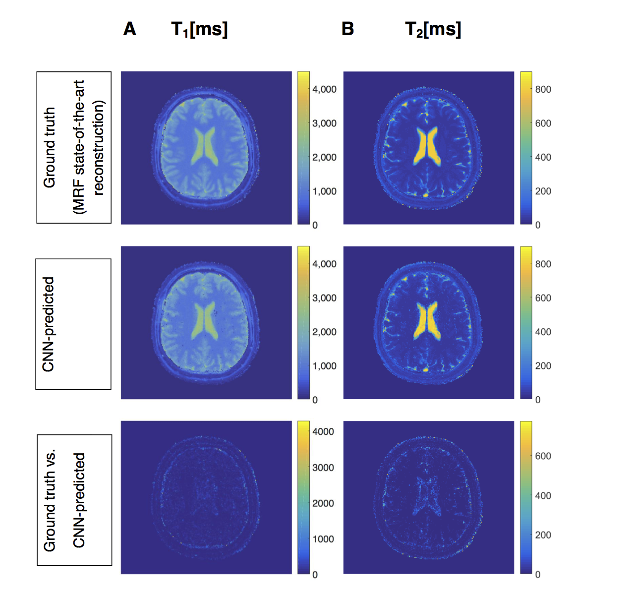
Figure 4: Prediction results from our proposed CNN in Figure 2 for human data. A: T1, B: T2. First row: Ground truth (state-of-the-art MRF reconstruction) quantitative relaxation maps, in units of ms. Second row: CNN-predicted quantitative relaxation maps, in units of ms. Third row: Absolute errors between ground truth and CNN-predicted relaxation maps, in units of ms. The results show, that our CNN was able to predict accurate quantitative T1 and T2 maps after training with human fingerprints, despite artifacts due to undersampling or other factors, e.g. movements of the living object of investigation.
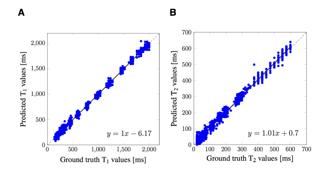
Figure 5: Results of predictions for one test ISMRM/NIST measurement (as in Figure 3) from a CNN with an architecture consisting of 4 layers (3 convolutional layers, average pooling and 1 fully-connected layer) as previously described for simulated data.5 A: T1, B: T2, in units of ms. The dashed line is the x=y line, the solid line is the linear regression (with its formula in the right corners). The results show, that a deeper architecture (compare to Figure 3, bottom row) was beneficial for predictions from measured fingerprints with undersampling artifacts, as a smaller architecture led to reduced accuracy.