2790
Deep Learning Reconstruction for Tailored Magnetic Resonance Fingerprinting1MIRC, Dayananda Sagar Institutions, Bangalore, India, 2MRI, GE Healthcare, Bangalore, India, 3Radiology, Columbia University, New York, NY, United States
Synopsis
Magnetic Resonance Fingerprinting (MRF) is an accelerated acquisition and reconstruction method employed to generate multiple parametric maps. Tailored MRF (TMRF) coupled with deep learning based reconstruction has been proposed to overcome the shortcoming of T2 under estimation and the need for dictionaries respectively. A generalized approach with training of natural images and a specific approach with training of brain data are detailed in this work. Both approaches are demonstrated, compared and quantified.
Purpose:
The aim of this work is to provide a dictionary-less approach to reconstruct multi-parametric MR maps based on Tailored Magnetic Resonance Fingerprinting acquisition method.Introduction:
Magnetic Resonance Fingerprinting (MRF) is an accelerated acquisition and reconstruction technique employed to generate multiple parametric maps1 Tailored MRF (TMRF) has been proposed with a block based (T1, T2 and PD) acquisition2 approach to overcome the limitation of under estimation of long T2 by dictionary resolution. To overcome this limitation, a deep learning based approach is proposed for the reconstruction of TMRF data. A three-layer Deep Neural Network (DNN) created on TensorFlow3 is used for training.Methods:
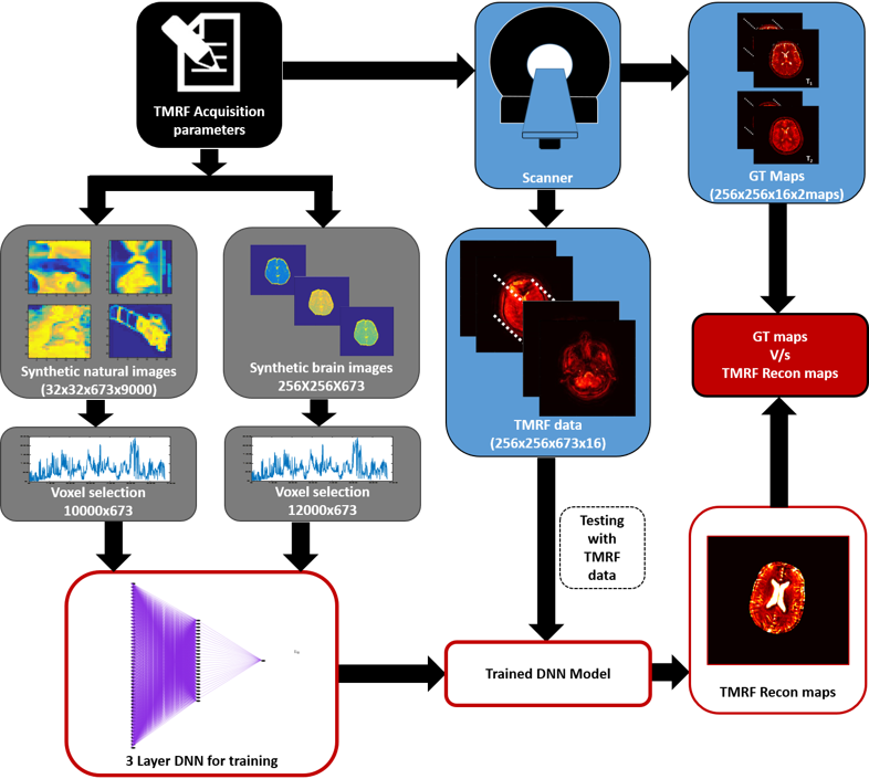
The reconstruction pipeline for tailored MRF using block based acquisition is demonstrated in Figure 1. Acquisition: The signal intensity of a gradient echo based sequence is more dependent on the Flip Angle (FA) than the Repetition Time (TR) due to the minimal TRs typically employed in such cases4. Thus, the required contrast can be achieved by an optimal choice of the FA. This has been utilized to form 3 blocks that optimize contrast for Proton Density (PD), T1 and T2 weighting. This allows each tissue type to have hyper-intensities in at least one of the three blocks. TRs and FAs were independently designed for each block and then combined into a single sequence. Each block comprised of 240 acquisitions (total of 720 TR/FA combinations). Four human in vivo brain data were acquired on a 1.5 T GE Signa with a spiral readout time of 5ms with a fixed Echo Time (TE) of 2.7ms, as part of an institution approved study. The spiral trajectory consisted of 48 arms and 720 images acquired using the TR/FA schedule was sliding window reconstructed to get 673 images. Training: We considered two approaches for general/brain specific image reconstruction. Approach 1: 10000 Natural images of size 32x32 were downloaded from CIFAR-10055 for training the NN. To improve the robustness of the proposed approach, 50% of the data was corrupted by introducing three artifacts: random rotation, Rician noise and circular shift because these discrepancies were commonly seen in TMRF data. As input to the Neural Network, 10000 voxels were randomly selected from synthesized data of size 32x32x673x10000 and trained against concurrent voxels selected from GT maps (T1 and T2). Approach 2: Synthetic brain images of size 128x128 were synthesized using the above method to create a training dataset of size 128x128x673. Similar to the previous approach, 12000 voxels were selected from the synthesized maps and GT maps (synthetic brain images) for NN training. The voxels selected were non-zero values selected from the region of the brain. DNN: T1 and T2 for approaches 1 and 2 were separately trained. A three layered DNN was used for both parameters. The DNN for T2 had weights of size 64, 32 and 1 for the layers, whereas the DNN for T1 had weights of size 128, 64 and 1. Testing: Voxel based testing was performed for both approaches on the data acquired using TMRF method. Four such datasets were used to test the DNN. The data was forward propagated through the trained NN to get the reconstructed voxels. These voxels were reshaped to generate reconstructed maps on Matlab (The Mathworks Inc, MA). The reconstructed maps were compared with the scanner generated GT maps to validate the proposed approaches. The code for this implementation is available online6.Results:
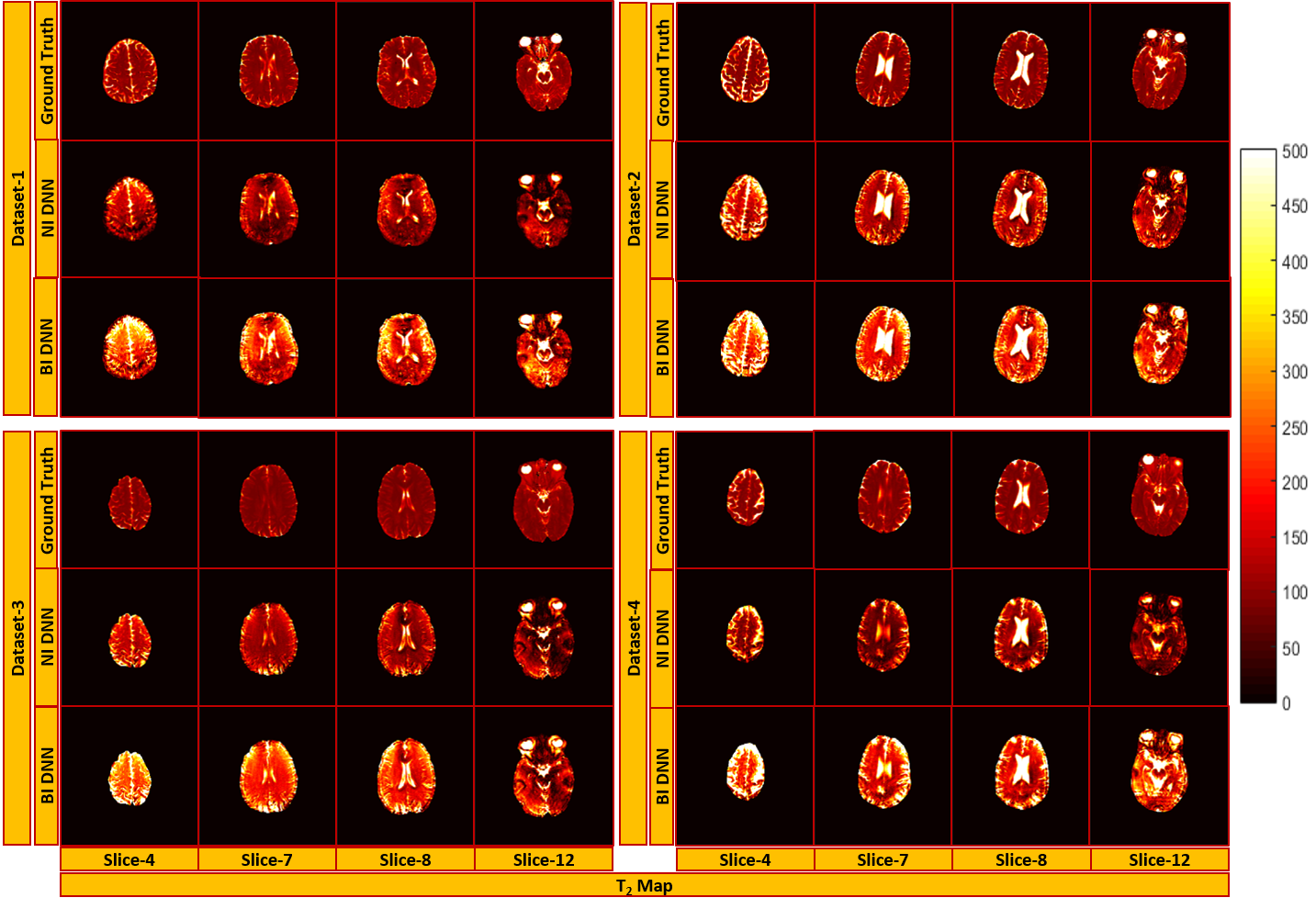
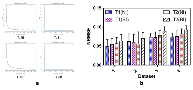
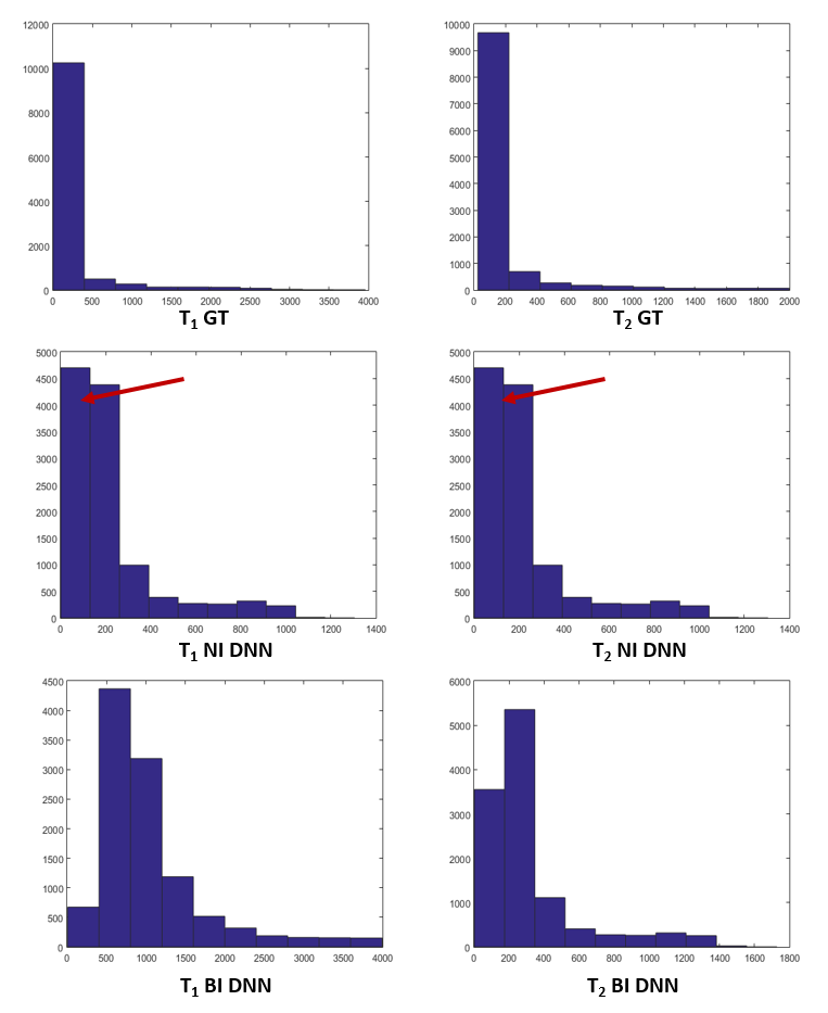
Figure 2 and 3 show the results of T1 and T2 from both approaches, compared with scanner generated GT maps respectively. Quantitative analysis for both the approaches is reported in Figure 4. A comparison of the learning curves (Figure 4(a)) shows the differences between the two approaches. Error between the reconstructed and scanner generated GT maps are calculated using Normalized Root Mean Square Error (NRMSE) metric. The graph shows that there is no significant difference between approach-1 and approach-2. However, Figure 5 illustrates the superior performance of the natural images based training over the other method through the retention of parametric values as indicated by the histograms. This is also reflected in Figures 2 and 3 over the four data sets.
Discussion and Conclusion
It can be ascertained that the results obtained from the first better compared to the second. We attribute this to the overfitting nature of the second neural network. This is also shown by the L-curves for training. A salient feature of the natural images approach is that it is not restricted to a single organ.Acknowledgements
This work was supported by Department of Science and Technology (DST) – DST/TSG/NTS/2013/100 and Vision Group on Science and Technology, Govt. of Karnataka, Karnataka Fund for strengthening infrastructure (K-FSIT), GRD#333/2015.References
[1]Dan Ma, et. al., Nature 2013
[2]Shaik Imam, et. al., ISMRM MRF workshop 2017
[3]Google inc., USA
[4] Brian Hargreaves, et. Al., JMRI 2012
[5] https://www.cs.toronto.edu/~kriz/cifar.html
[6]https://github.com/mirc-dsi/IMRI MIRC/tree/master/MR%20RECON/CODE/TMRF_DNN_Recon
Figures