2787
Synthetic CT Generation using MRI with Deep Learning: How does the selection of input images affect the resulting synthetic CT?1Department of Radiology and Biomedical Imaging, University of California San Francisco, San Francisco, CA, United States, 2UC Berkeley - UC San Francisco Joint Graduate Program in Bioengineering, Berkeley and San Francisco, CA, United States
Synopsis
Most recently, synthetic CT generation methods have been utilizing deep learning. One major open question with this approach is that it is not clear what MRI images would produce the best synthetic CT images. We investigated how the selection of MRI inputs affect the resulting output using a fixed network. We found that Dixon MRI may be sufficient for quantitatively accurate synthetic CT images and ZTE MRI may provide additional information to capture bowel air distributions.
Introduction
Four different MRI protocols are typically used for synthetic CT generation: conventional T1- or T2-weighted MRI1,2, Dixon MRI3, UTE MRI4, and ZTE MRI5. The major advantage of using Dixon MRI, UTE MRI, and ZTE MRI over conventional MRI is that they have been found to have signal intensity correlations with Hounsfield units.
Various image processing and machine learning methods have been used to turn these MRI images into synthetic CT images6. Most recently, synthetic CT generation methods have been utilizing deep learning1,2,7. One major open question with this approach is that it is not clear what MRI images would produce the best synthetic CT images. This work uses different combinations of input images with deep learning and assesses the resulting synthetic CT images. This work is focused on the pelvis, where synthetic CTs are useful for evaluation of prostate cancer and other pelvic malignancies.
Methodology
Patients with pelvis lesions were scanned using an integrated 3 Tesla time-of-flight (TOF) PET/MRI system8 (SIGNA PET/MR, GE Healthcare, Waukesha, WI, USA). Ten patients were used for training and sixteen patients were used for validation.
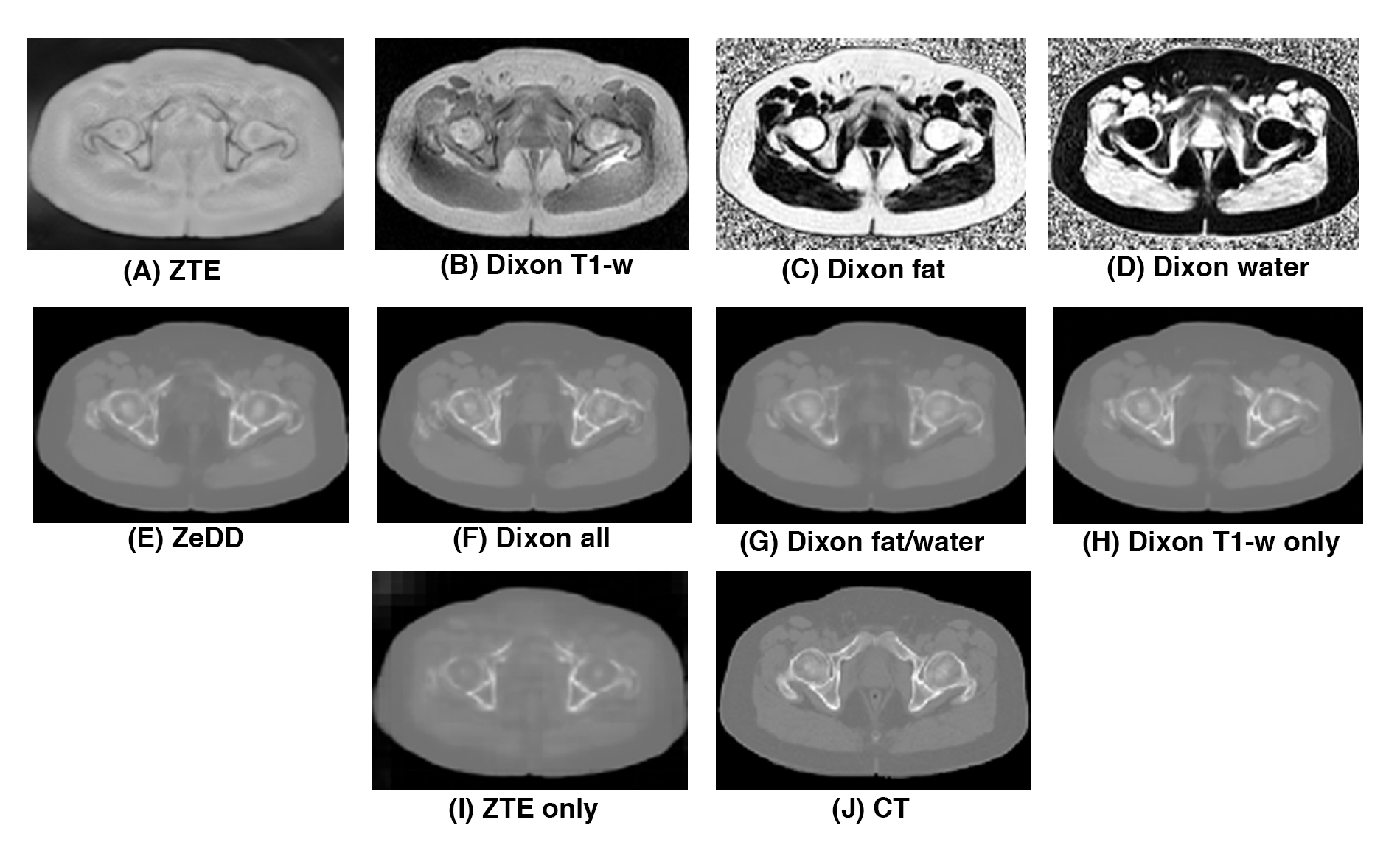
Figure 1 shows the different MRI inputs used for this work: bias-corrected soft-tissue normalized proton-density-weighted ZTE, bias-corrected and fat-peak normalized Dixon T1-weighted image, Dixon fractional fat map, and Dixon fractional water map.
A previously-published deep convolutional neural network for synthetic CT generation was used7 and the same training methodology and synthetic CT generation for the network was performed. The combinations of MRI inputs used were as follows:
- ZTE + Dixon fractional fat + Dixon fractional water (ZeDD)7
- ZTE only
- Dixon T1-w + Dixon fractional fat + Dixon fractional water (Dixon all)
- Dixon T1-w only
- Dixon fractional fat + Dixon fractional water (Dixon fat/water)
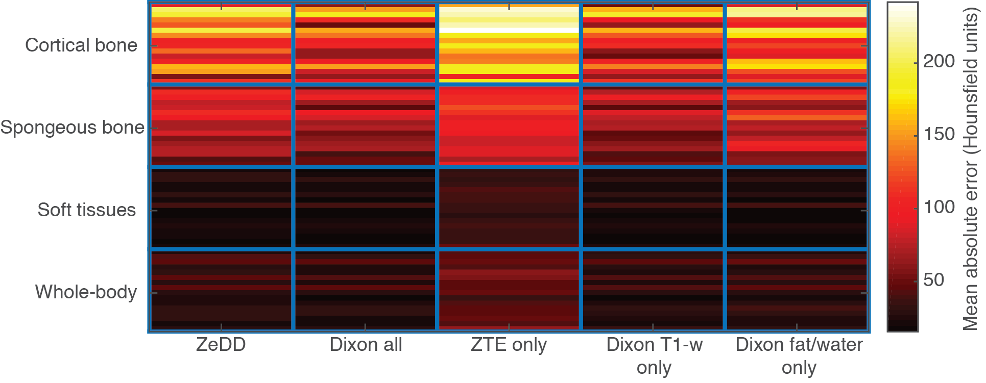
Qualitative analysis of the training curves of the different combinations of MRI inputs was performed and visual inspection of the synthetic CT images was performed. The quantitative analysis of the synthetic CT images was performed only in body voxels (synthetic CT > -120 HU AND CT > -120 HU) to eliminate any errors due to air mismatch. The mean absolute error was measured over the whole pelvis, in soft-tissues (-120 to 100 HU), in spongeous bone (100 to 300 HU), and cortical bone (> 300 HU) across the validation dataset. Additionally, the synthetic CT images were down-sampled to a resolution of 4.69×4.69×2.81mm and filtered with a 10mm Gaussian kernel to simulate the pre-processing step used for producing PET/MRI attenuation coefficient maps.
Results
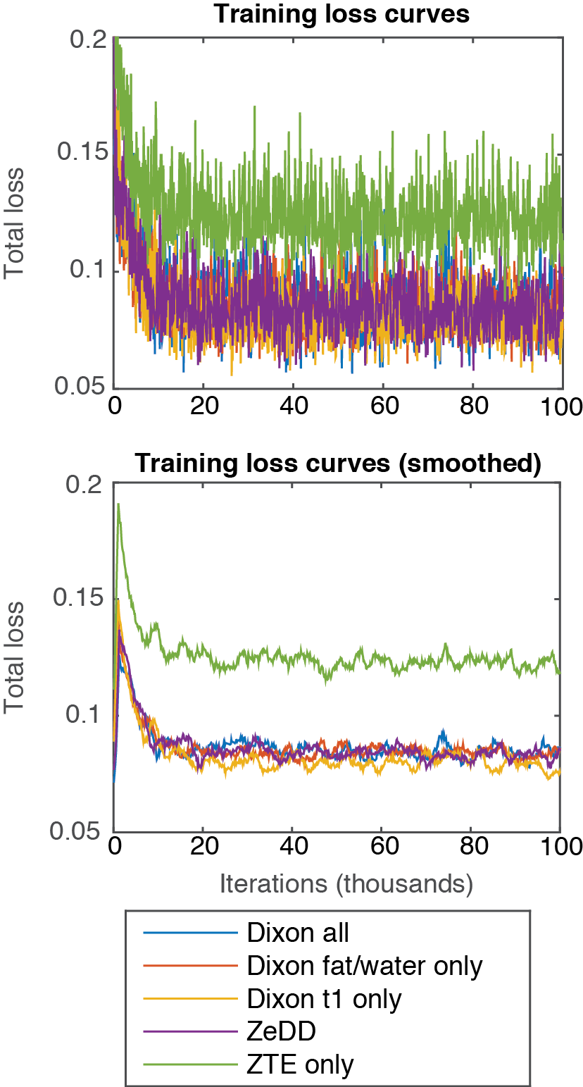
Figure 2 shows the training curves for each combination of MRI inputs. Each training converged at approximately 20 thousand iterations. ZTE-only inputs achieved the highest training loss while all other inputs provided very similar training behaviors at about 0.7 training loss.
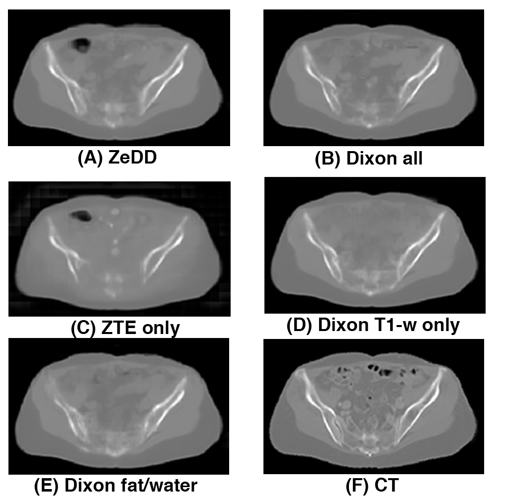
Figure 3 shows the synthetic CT images produced with the different combinations of MRI inputs and the ground- truth CT for one patient in the validation set. All other synthetic CT methods provided excellent depiction of soft-tissues and bone except for ZTE-only. Only the ZTE-based methods were able to produce bowel air in the synthetic CT images. Example images for another patient in the validation set is shown in Figure 4.
Figure 5 shows the mean absolute error of each synthetic CT compared to ground-truth CT. In each specific tissue compartment, ZTE-only had the largest errors. For the other synthetic CT images, ZeDD, Dixon all, Dixon T1-w only, and Dixon fat/water only were comparable in the soft-tissue compartments. Dixon all and Dixon T1-w were comparable in bone compartments and had less error than ZeDD and Dixon fat/water.
Discussion
Several groups have now demonstrated that deep learning can effectively produce synthetic CT images from MRI. This work evaluates what types of MRI inputs are required. We found that, in the pelvis, using only T1-weighted MRI as the input was effective at generating synthetic CT. This was a surprising result, as we expected ZTE MRI would provide additional bone information that could improve the synthetic CT. One possible explanation is that the bone regions on T1-weighted MRI in the pelvis are well-defined by the lack of signal, and thus the non-zero signal in bone with ZTE MRI is not required.Conclusion
We investigated the effects of having different combinations of MRI inputs to generate synthetic CT images with a deep convolutional neural network model. We found that, in the pelvis, Dixon MRI may be sufficient to produce quantitatively accurate synthetic CT images.Acknowledgements
The authors of this work received research funding from GE HealthcareReferences
[1] D. Nie, X. Cao, Y. Gao, L. Wang, and D. Shen, “Estimating CT Image from MRI Data Using 3D Fully Convolutional Networks,” in Deep Learning and Data Labeling for Medical Applications, 2016, pp. 170–178.
[2] F. Liu, H. Jang, R. Kijowski, T. Bradshaw, and A. B. McMillan, “Deep Learning MR Imaging–based Attenuation Correction for PET/MR Imaging,” Radiology, p. 170700, Sep. 2017.
[3] S. D. Wollenweber et al., “Comparison of 4-Class and Continuous Fat/Water Methods for Whole-Body, MR-Based PET Attenuation Correction,” IEEE Transactions on Nuclear Science, vol. 60, no. 5, pp. 3391–3398, Oct. 2013.
[4] C. N. Ladefoged et al., “Region specific optimization of continuous linear attenuation coefficients based on UTE (RESOLUTE): application to PET/MR brain imaging,” Phys. Med. Biol., vol. 60, no. 20, p. 8047, 2015.
[5] A. P. Leynes et al., “Hybrid ZTE/Dixon MR-based attenuation correction for quantitative uptake estimation of pelvic lesions in PET/MRI,” Med. Phys., vol. 44, no. 3, pp. 902–913, Mar. 2017.
[6] C. N. Ladefoged et al., “A multi-centre evaluation of eleven clinically feasible brain PET/MRI attenuation correction techniques using a large cohort of patients,” NeuroImage, vol. 147, pp. 346–359, Feb. 2017.
[7] A. P. Leynes et al., “Direct PseudoCT Generation for Pelvis PET/MRI Attenuation Correction using Deep Convolutional Neural Networks with Multi-parametric MRI: Zero Echo-time and Dixon Deep pseudoCT (ZeDD-CT),” J Nucl Med, p. jnumed.117.198051, Oct. 2017.
[8] C. S. Levin, S. H. Maramraju, M. M. Khalighi, T. W. Deller, G. Delso, and F. Jansen, “Design Features and Mutual Compatibility Studies of the Time-of-Flight PET Capable GE SIGNA PET/MR System,” IEEE Transactions on Medical Imaging, vol. 35, no. 8, pp. 1907–1914, Aug. 2016.
Figures