Synopsis

A new approach to auto-calibrating, coil-by-coil parallel imaging reconstruction is presented. It is a generalized reconstruction framework based on deep learning. A neural network consisting of three Dense layer (Fully connected layer) units, an RNN layer and an output Dense unit is designed and trained to identify the mapping relationship between the zero-filled and fully-sampled k-space data. The training process could be separated into two steps: pre-training and fine-tuning. Results show our proposed model could be robust to arbitrary undersampling patterns in k-space and shows a higher structural similarity index compared with traiditional k-space based methods.

Introduction

Parallel imaging is a common approach to accelerate the MRI acquisition by exploiting the data redundancy in multiple coil scans ^1-3. Several other strategies, like compressed sensing (CS)^4-6, have been proposed to achieve more aggressive undersampling factors, and deep learning is also capable of obtaining prior knowledge with the help of training datasets for MR image reconstruction. Many attempts have been carried out to automate image reconstruction by learning historical datasets ^1,7-9 and have focused on image domain, aiming to remove the aliasing artifacts using convolutional neural network (CNN). In this work, we implement auto-calibrated image reconstruction from the k-space domain using a fully connected recurrent neural network (FC-RNN network).

Theory and Methods

In GRAPPA ¹¹, unacquired k-space data in the $$$i^{th}$$$ coil, at position $$$r$$$, $$$x_i\left( r \right) $$$, can be synthesized by a linear combination of acquired neighboring k-space data from all coils. Let $$$\tilde{R}_r$$$ be the operators that chooses a smaller subset of only the acquired k-space locations in the neighborhood of $$$r$$$ . The recovery of $$$x_i\left( r \right) $$$ is given by:

$$x_i\left( r \right) =\sum_j{g_{r\ ji}\left( \tilde{R}_rx_j \right)}$$

where $$$g_{r\ ji}$$$ is a vector set of weights obtained by calibration for the particular sampling pattern around $$$r$$$.

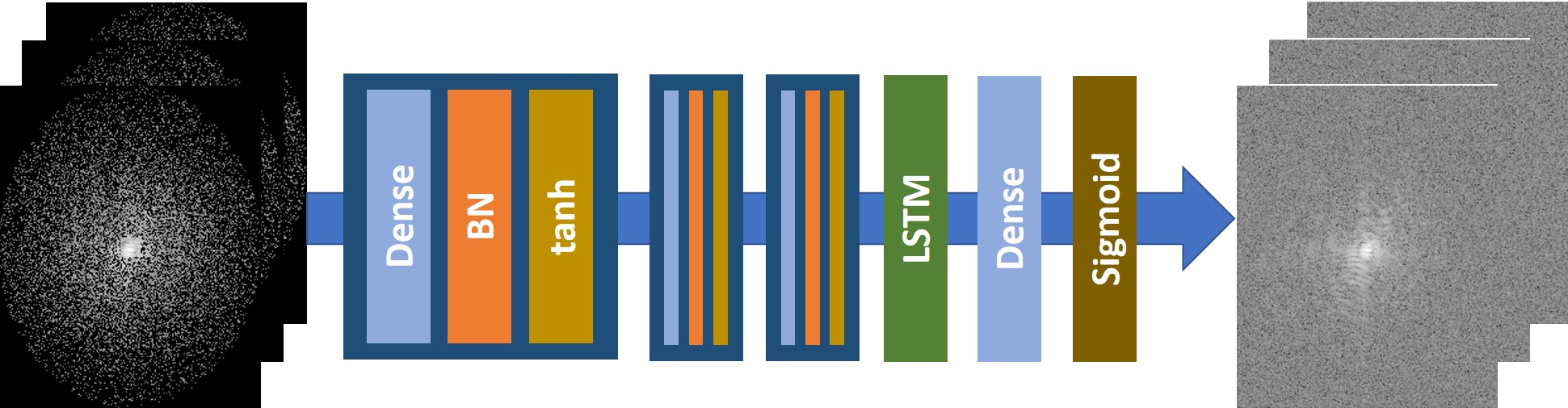
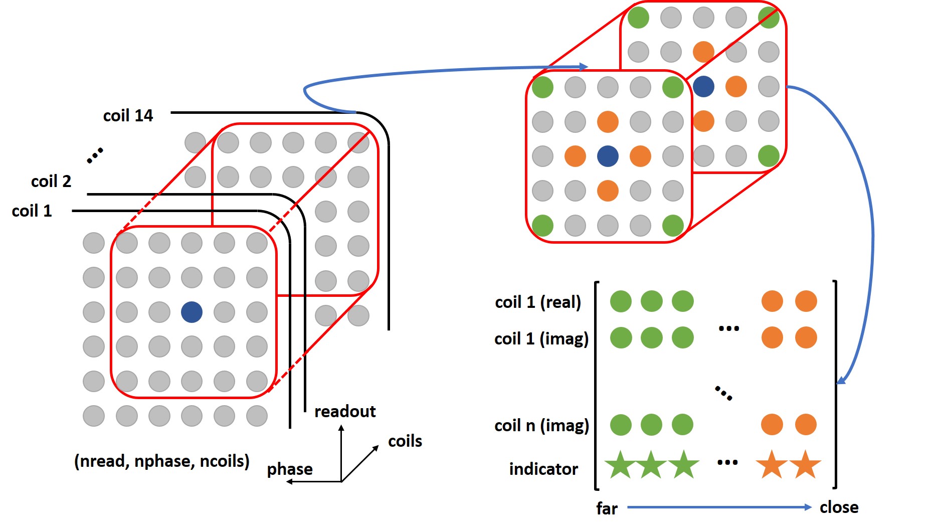
Instead of using a linear operator, the deep neural network can be used to estimated unacquired k-space data using a non-linear mapping. Our proposed FC-RNN architecture is shown in Fig.1, consisting of three dense units, an LSTM layer and an output dense unit. Firstly, the input data (a $$$5\times5$$$ block with $$$14$$$ coils) need to be reshaped into a 2D matrix, where the 2D matrix was organized by their distance from the data to be reconstructed (blue circle). The green circles, far from blue, were placed at the beginning of the 2D matrix, while the orange circles, close to blue, were placed at the end (Fig. 2). To account for complex numbers, the k-space data were split into real and imaginary parts, and separate FC-RNNs were used for real and imaginary parts. Finally, a binary indicator was used for each k-space position, indicating whether it was acquired or not. After reorganization, all the input data and output data were normalized into $$$\left[ 0,1 \right]$$$ for improved network performance.

The training process consisted of two independent steps, pre-training and fine-tuning. We used a large dataset (volunteer scans from Siemens 3T Prisma scanner, with T1 vibe water excitation breath-hold sequence) for pre-training, and fine-tuning was performed for each data set using on the auto-calibration area. For training, both steps were applied to the specific undersampling patterns, and for reconstruction, a sliding block traversed through the entire k-space was fed into the deep network after reorganizing the block, as illustrated in Fig. 2.

Results and Discussion

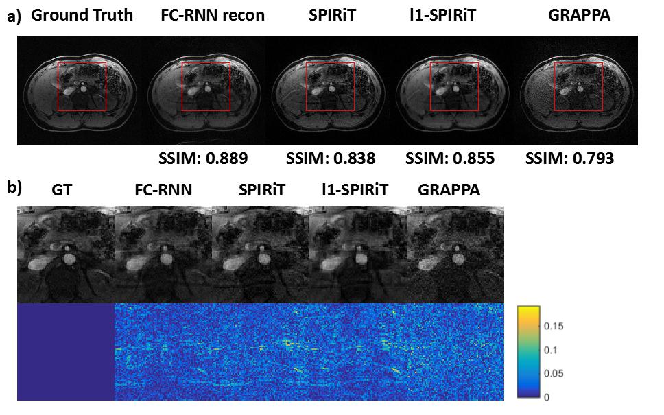
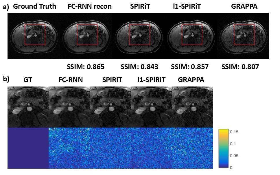
Since our model is designed for arbitrary k-space undersampling patterns, both uniform and random ones are tested with our proposed method. Other kspace self-autocalibration methods, including SPIRiT, $$$l_1$$$-SPIRiT and GRAPPA have also been adopted for comparison. The undersampling masks could be seen in Fig. 3, which includes a $$$3\times$$$ uniform sampling and a $$$4\times$$$ random sampling. The abdominal dataset was obtained fully-sampled with $$$14$$$-channel coil and $$$256\times208$$$ matrix. In the uniform undersampling case, as shown in Fig. 4, our proposed method produces shallower artifacts and has an edge in the error map compared to SPIRiT and -SPIRiT. Moreover, different from the rough images produced by GRAPPA, zoom-in image shows FC-RNN result is capable of preserving fine structures of the original image. This kind of characteristic has made it appear more natural in detail, which could also be concluded from the SSIM(structural similarity) index. Referring now to Fig. 5, although CS based methods naturally fits the random pattern quite well, our approach is able to produce a similar result without explicitly applying CS theory and has maintained its advantage in SSIM index.

Conclusions and Future Work

Acknowledgements

References

1. Lustig M, Pauly J M. SPIRiT: Iterative self‐consistent parallel imaging reconstruction from arbitrary k‐space. Magnetic resonance in medicine, 2010, 64(2): 457-471.
2. Knoll F, Clason C, Bredies K, et al. Parallel imaging with nonlinear reconstruction using variational penalties. Magnetic Resonance in Medicine, 2012, 67(1): 34-41.
3. Schlemper J, Caballero J, Hajnal J V, et al. A Deep Cascade of Convolutional Neural Networks for Dynamic MR Image Reconstruction. arXiv preprint arXiv:1704.02422, 2017.
4. Lingala S G, Hu Y, DiBella E, et al. Accelerated dynamic MRI exploiting sparsity and low-rank structure: kt SLR. IEEE transactions on medical imaging, 2011, 30(5): 1042-1054.
5. Haldar J P, Liang Z P. Spatiotemporal imaging with partially separable functions: A matrix recovery approach. Biomedical Imaging: From Nano to Macro, 2010 IEEE International Symposium on. IEEE, 2010: 716-719.
6. Lustig M, Donoho D L, Santos J M, et al. Compressed sensing MRI. IEEE signal processing magazine, 2008, 25(2): 72-82.
7. Hyun C M, Kim H P, Lee S M, et al. Deep learning for undersampled MRI reconstruction. arXiv preprint arXiv:1709.02576, 2017.
8. Mardani M, Gong E, Cheng J Y, et al. Deep Generative Adversarial Networks for Compressed Sensing Automates MRI. arXiv preprint arXiv:1706.00051, 2017.
9. Sun J, Li H, Xu Z. Deep ADMM-net for compressive sensing MRI. Advances in Neural Information Processing Systems. 2016: 10-18.
10. Wang Z, Bovik A C, Sheikh H R, et al. Image quality assessment: from error visibility to structural similarity[J]. IEEE transactions on image processing, 2004, 13(4): 600-612.
11. Griswold M A, Jakob P M, Heidemann R M, et al. Generalized autocalibrating partially parallel acquisitions (GRAPPA). Magnetic resonance in medicine, 2002, 47(6): 1202-1210.