2783
Deep Generative Adversarial Networks for High Resolution fMRI using Variable Density Spiral Sampling1Center for Biomedical Imaging Research, Department of Biomedical Engineering, School of Medicine, Tsinghua University, Beijing, China, 2University of Oxford, London, United Kingdom
Synopsis
An approach to fMRI image reconstruction for variable density radial trajectories is proposed in this abstract. We have employed Generative Adversarial Networks (GAN), which is made up of a generator and a discriminator, to map input aliasing images to gold standard images. Different from the large computation requirements of CS-based methods, the proposed method is able to both boost reconstruction efficiency and achieve a good image quality in the meantime.
Introduction
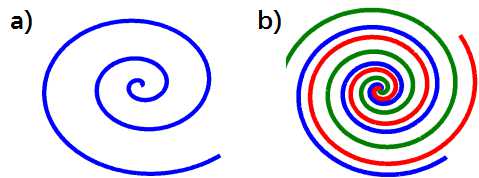
Functional magnetic resonance imaging (fMRI) requires efficient acquisition methods in order to fully sample the brain in a several-second time period 1. The spiral method,as shown in Fig. 1, samples k-space with an Archimedean or similar trajectory and is widely acknowledged for its shorter readout times and improved signal recovery. However, multi-shot spiral is often needed for increasing interest in higher resolution fMRI, which inevitably results in longer readout duration. Parallel imaging 2 and compressed sensing (CS) techniques 3 have already been applied in exploiting the redundancy in MR data, and deep learning is also capable of utilizing prior knowledge with the learning process of historical dataset. In this abstract, we would present a deep generative adversarial network which is able to restore high resolution image with a small subset of trajectories.Theory and methods
Consider a linear system $$$y=\varPhi x$$$, where $$$\varPhi$$$ refers to the specific sampling trajectory. Let $$$R$$$ represent an operator that chooses a small subset of all the trajectories, the undersampled image $$$x$$$ could be written as:
$$x=\varPhi ^{-1}\left\{ R\left[ \varPhi \left( y \right) \right] \right\} $$
In this case, $$$\varPhi$$$ specifically represents the NUFFT transform. Given an observation $$$x$$$, our goal is to reconstruct $$$\hat{y}$$$ that resembles $$$y$$$.
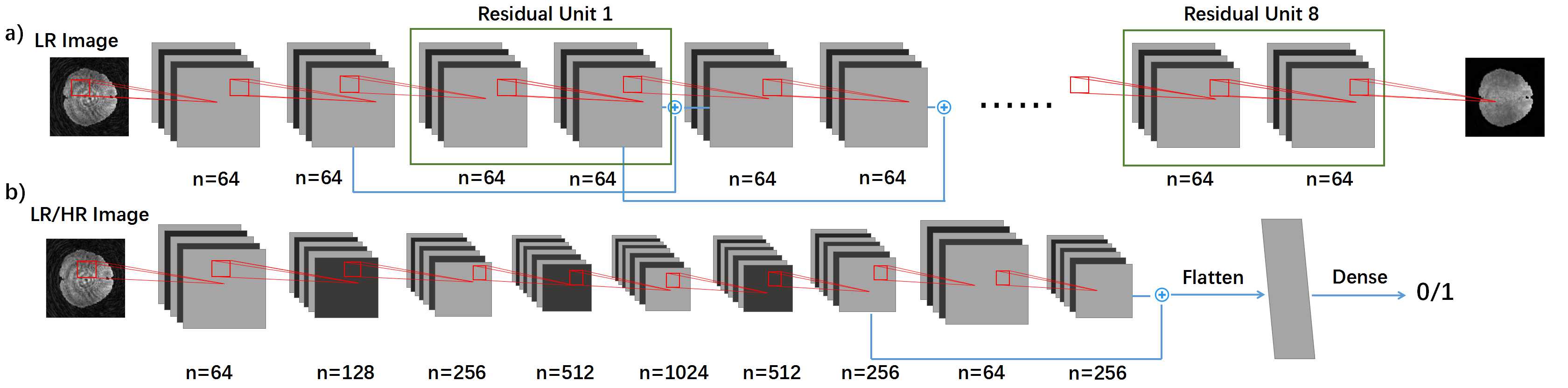
As stated above, a generative adversarial network has been employed to solve the inversion recovery problem. As shown in Fig.2 , it consists of two separate networks: generator $$$G$$$ and discriminator $$$D$$$. The low resolution, aliasing image $$$x$$$ would be fed into the generator and the output would be the estimation $$$\hat{y}$$$. The main task of discriminator $$$D$$$, on the other side, would be to check if $$$\hat{y}$$$ belongs to high quality images $$$Y$$$. The training process for the network amounts to be a game with conflicting objects between $$$D$$$ and $$$G$$$. The network $$$D$$$ aims to tell real images from estimations generated by $$$G$$$, whereas $$$G$$$ hopes to map input image $$$x$$$ to real-life image and fool $$$D$$$. In this way, the training loss could be written as:
$$L_D=E\left[ \left( 1-D\left( y;\varTheta d \right) \right) ^2 \right] +E\left[ D\left( \hat{y};\varTheta d \right) ^2 \right] $$
$$L_G=E\left[ \left( 1-D\left( G\left( x;\varTheta _g \right) ;\varTheta _d \right) \right) ^2 \right]$$
However, for the generated images classified as the real with high confidence, no loss would occur and the generator may introduce non-realistic images 4. Hence we would adopt a mixture of discriminator scoring, pixel-wise loss and data consistency term in training generator $$$G$$$:
$$L_G=E\left[ \left( 1-D\left( G\left( x;\varTheta _g \right) ;\varTheta _d \right) \right) ^2 \right] +\lambda _1\left( \lVert G\left( x;\varTheta _g \right) -y \rVert _2 \right) +\lambda _2\left( \lVert R\varPhi \left( G\left( x;\varTheta _g \right) \right) -R\varPhi \left( y \right) \rVert _1 \right) $$
Note the second term in the above equation represents the mean squared error between the generated image and ground truth, while the third one refers to a soft penalty that ensures the input to network D is data consistent.
Results and Discussion
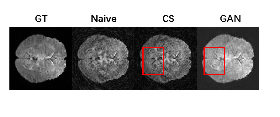
The network is trained on an fMRI dataset with Adam optimizer and an initial learning rate of $$$l_r=10^{-3}$$$. The data were acquired on a Philips 3.0T Achieva TX MRI scanner (Philips Healthcare, Best, The Netherlands) using a 32-channel head coil with Golden angle rotated variable density spiral (VDS) (α=4) sampling. Training is implemented with TensorFlow on NVIDIA GeForce GTX 1080 Ti. The reconstruction results with 2 leaves of 20 in total ($$$\times10$$$ undersampling) can be seen in Fig. 3 together with CS-based approaches and naive (direct) reconstruction. As shown in the figure, our method is able to reduce spiral artifacts as well as preserving fine structures of the original image (especially in the red rectangle area). The conclusion can also be drawn from Tab. 1, in which the GAN based method is significantly better in terms of SSIM and SNR. Last but not least, the time efficiency of this approach would make it possible for real time scans.Conclusion
This paper proposes a novel GAN network that leverages historical data for more diagnosis-valuable image reconstruction from highly undersampled observations. The neural network is trained to map a readily obtainable undersampled image to the corresponding high resolution one with the constraint of data consistency. Experiment results based on fMRI dataset shows our method is able to generate images with better quality in a real-time manner (about 10 times faster), which could hopefully enhances its use in clinical scenarios. Future work may focus on applying time-frame correlations for improved quality and robustifying against patients with abnormalities.Acknowledgements
No acknowledgement found.References
- Glover, Gary H. "Spiral imaging in fMRI." Neuroimage 62.2 (2012): 706-712.
- Law, Christine S., Chunlei Liu, and Gary H. Glover. "Sliding‐window sensitivity encoding (SENSE) calibration for reducing noise in functional MRI (fMRI)." Magnetic resonance in medicine60.5 (2008): 1090-1103.
- Feng, Li, et al. "Golden‐angle radial sparse parallel MRI: Combination of compressed sensing, parallel imaging, and golden‐angle radial sampling for fast and flexible dynamic volumetric MRI." Magnetic resonance in medicine 72.3 (2014): 707-717.
- Mao X, Li Q, Xie H, et al. Least squares generative adversarial networks. arXiv preprint ArXiv:1611.04076, 2016.
- Wang Z, Bovik A C, Sheikh H R, et al. Image quality assessment: from error visibility to structural similarity[J]. IEEE transactions on image processing, 2004, 13(4): 600-612.
Figures