Synopsis

The MRF framework has significant freedom in sequence design, increasing its utility and scope, but also the difficulty of determining an optimally efficient experiment. To address this challenge, a statistical analysis of MRF is used to develop a model relating the error in relaxation time quantification and the resulting experimental efficiencies to the number of repetitions in a FISP-MRF experiment. In general, T­­₁ and T₂ efficiencies peak prior to 1000 time steps, then decrease to constant values for larger time step totals. Therefore, the derived model can be used to design efficient MRF experiments.

Purpose

Methods

To understand FISP-MRF statistics, a model is derived for a simple experiment, then applied to experiments with varying input parameters.

Using analysis presented in Kara et al.,¹ the MRF signal as a function R₁=1/T₁ and R₂=1/T₂ is modeled by a Taylor series expansion. Then, a dictionary entry corresponding to R₁ and R₂ is $$$\overrightarrow{D}\left(R_{1},R_{2}\right)\cong\overrightarrow{C}_{0}+\overrightarrow{C}_{1}\left(R_{1}-R_{1,0}\right)+\overrightarrow{C}_{2}\left(R_{2}-R_{2,0}\right)$$$ and a noisy signal with underlying R_1,0 and R_2,0 is $$$\overrightarrow{S}\cong\overrightarrow{C}_{0}+\overrightarrow{\eta}$$$, where $$$\overrightarrow{C}_{0}=\overrightarrow{D}\left(R_{1,0},R_{2,0}\right)$$$ and $$$\overrightarrow{C}_{i}=\frac{\partial\overrightarrow{D}}{\partial R_{i}}\mid_{R_{1}=R_{1,0},R_{2}=R_{2,0}}$$$ for i=1,2. Then, error due to noise in mapping R_i is $$\sigma_{R_{i}}^{2}=\sigma_{\eta}^{2}/Q_{i} \quad (i=1,2) \qquad (1)$$ where Q_i is a function of $$$\hat{C}_{0}, \hat{C}_{1}$$$, and $$$\hat{C}_{2}$$$.¹

For a simple experiment (constant flip angle, TR), $$$\overrightarrow{C}_{0}, \overrightarrow{C}_{1}$$$, and $$$\overrightarrow{C}_{2}$$$ become constant in the steady state. Therefore, $$\hat{C}_{j}=\frac{\overrightarrow{C}_{j}}{\sqrt{c_{j}+ C_{j,ss}^{2}N}} \quad \left(j=0,1,2\right)\qquad (2)$$ with constant c_j and total number of acquired time steps N. Then, using Eq. (2), $$Q_{i}=\frac{\sum_{k=0}^{3}\alpha_{i,k}N^{k}}{\sum_{l=0}^{2}\beta_{i,l}N^{l}} \quad (i=1,2) \qquad (3)$$ where coefficients $$$\alpha_{i,k}$$$ and $$$\beta_{i,l}$$$ depend on the imaging sequence. In the large N limit, Eq. (3) implies that Q_i becomes proportional to N; thus, $$$\sigma_{R_{i}}$$$ approaches $$$\sqrt{N}$$$, the expected statistical result for N repeated, independent experiments.

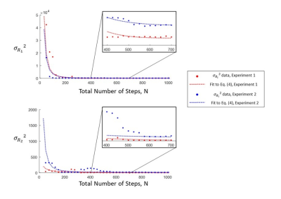
This model was tested in multiple FISP-MRF simulations and experiments, with varying flip angle distributions, constant TR and TE (6.98ms, 2.93ms), and N up to 10000 steps. The numerator of Q_i is dominated by $$$\alpha_{i,2}N^{2}$$$ for clinically relevant values of N (<3,000 steps), so that $$\sigma_{R_{i}}^{2}\cong a_{i,0}+\frac{a_{i,1}}{N}+\frac{a_{i,2}}{N^{2}} \quad(i=1,2)\quad [N<3000] \qquad (4)$$

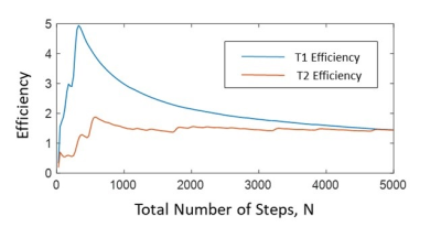
Simulated Q_i for various FISP-MRF sequences reveal rapid increases in Q_i early in the first 1000 repetitions, beyond which growth in Q_i slows to the linear relationship in N predicted by Eq.(3). Therefore, the efficiency of a FISP-MRF experiment in mapping T_i, assuming approximately constant TR, is expected to be greatest prior to linear growth, after which the efficiency becomes approximately constant according to² $$Efficiency=\frac{T_{i}}{\sigma_{T_{i}}\sqrt{T_{seq}}} \quad (i=1,2) \qquad (5)$$

The efficiencies of three experiments of differing durations and/or acceleration factors are compared. Flip angle distributions based on Jiang et al.³ with constant TR (6.98ms) and TE (2.93ms) were used to image a 10 compartment phantom on a 3T Siemens Skyra. In cases 1 (Standard Experiment) and 2 (Fast Experiment), 1000 and 500 time points were collected with a single-shot variable density spiral to produce undersampled (R=48) data sets in 6980s and 3490s respectively. In case 3 (Double-Shot Experiment), 500 time points were collected with two spiral interleaves per time step (30s between acquisitions), to produce an undersampled (R=24) data set in 7010s. Monte-Carlo bootstrapping was used to calculate $$$/sigma_{R}_{i}^{2}$$$ per voxel, from which average $$$/sigma_{R}_{i}^{2}$$$ was calculated over 5x5 ROIs.⁴

Results and Discussion

Fits of simulated Q_i and experimental data using Eqs.(3) and (4) from two experiments, both with flip angle distributions based on Jiang et al., are presented in Figs. [1] and [2] respectively. Experiment 1 uses an initial inversion pulse, and Experiment 2 uses intermittent preparation pulses.⁵ In both cases, rapid increases in Q_i, reflected by rapid decreases in experimental occur prior to N=1000, followed by linearity in N. Although intermittent preparation pulses do not affect linearity, the Q­_i­ and N proportionality is increased, resulting in lower $$$\sigma_{R_{i}}^{2}$$$.

In Fig. [3], the T­₁ and T­₂ efficiency of Experiment 1 is calculated from Q­_i data for varying values of N, assuming $$$T_{seq}=N \cdot TR$$$ (constant TR=6.98ms). An initial efficiency spike is followed by constant efficiency as Q_­i becomes linear in N.

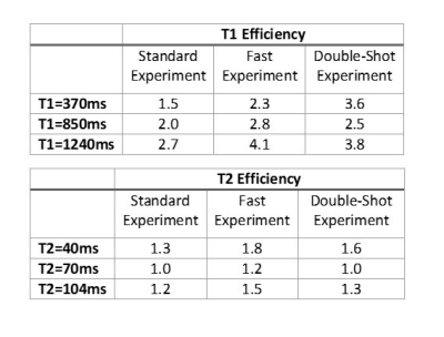
Table 1 displays the Standard, Fast, and Double-Shot efficiencies for three phantom ROIs. The Standard is least efficient in all phantom ROIs, and the Fast is, in general, most efficient. On average, the Fast (Double-Shot) offers a 39% (25%) improvement in T­₁ efficiency and a 26% (25%) improvement in T₂ efficiency relative to the Standard. That the Standard is least efficient agrees with the presented statistical model. Increased efficiency for the Fast compared to the Double-Shot suggests the aliasing noise decrease using two rather than one k-space interleaves per step is insufficient to warrant the increased acquisition time.

Conclusion

Acknowledgements

References

[1] Kara D, et al. Proc. ISMRM 2017:1350.

[2] Ma D, et al. Nature 495, 187-92 (2013).

[3] Jiang Y, et al. MRM 74:1621–1631 (2015).

[4] Riffe M J et al. Proc. ISMRM 2017:1879.

[5] Hamilton J et al. MRM doi:10.1002/mrm.26216.