2778
Physical parameterization of relaxation curves in GRE sequences1Dept.of Radiology, Medical Physics, Medical Center University of Freiburg, Faculty of Medicine, University of Freiburg, Freiburg, Germany
Synopsis
The parameter T2* is often used to describe the apparent rate of spin-spin relaxation in the presence of local magnetic field gradients, which is commonly assumed to be mono-exponential. However, the behavior of the transverse relaxation is more complex, since structural characteristics of biological tissues are encoded in the shape of relaxation curve which cannot be described by a single parameter. Several attempts have been made to introduce more accurate relaxation models. In this work we present a concept for the quantitative analysis of the relaxation curve shape in gradient-recalled echo (GRE) imaging based on physical parameters of the signal.
Introduction
The parameter T2* is often used to describe the apparent rate of spin-spin relaxation in the presence of local magnetic field gradients. It is calculated by fitting a mono-exponential function onto the relaxation curve. However, the behavior of the transverse relaxation is more complex than mono-exponential, as e.g. structural characteristics of biological tissues are encoded in the shape of relaxation curve which cannot be described by a single parameter T2* alone [1-7]. In the presence of mesoscopic local magnetic field gradients and T2 heterogeneities, T2* values are often misleading as they strongly depend on the location in the patient. Several attempts have been made to introduce more accurate relaxation models [8-10]. In this work we present a concept for the quantitative analysis of the relaxation curve shape in gradient-recalled echo (GRE) imaging based on a more detailed 3D analysis of the signal relaxation curve.Methods
In our spin relaxation model, we define a set of numerical parameters to characterize the tissue structure and to describe the unique relaxation curve shape in each voxel. The following analytical formula for signal relaxation within a voxel has been derived from this model:
$$S(t)=S_{0}v\cdot e^{-t/T_{2}}\cdot R_{p_{x}}(\alpha_{x} t)\cdot R_{p_{y}}(\alpha_{y} t)\cdot R_{p_{z}}(\alpha_{z} t), \hspace{2mm} R_{p}(x)=\frac{1}{x}\int_{0}^{x} \cos(pu)e^{-u^{2}}du,\hspace{2mm}(1)$$
where
$$\alpha_{x,y,z}=\frac{\gamma}{4}\sigma_{x,y,z}l_{x,y,z},\hspace{2mm} p_{x,y,z}=\frac{2\overline{G}_{x,y,z}}{\sigma_{x,y,z}}.\hspace{2mm}(2)$$
Here, $$$l_{x,y,z}$$$ are the voxel dimensions, $$$v$$$ is the voxel volume, $$$\overline{G}_{x,y,z}$$$ are the average values of the magnetic field gradients with standard deviations $$$\sigma_{x,y,z}$$$. Equation (1) cannot be fitted effectively, but a simplified version, which is a 3D generalization of the Hahn relaxation formula [11] GRE signal:
$$S(t)=S_{0}\cdot\exp\left[-\frac{t}{T_{2}}-(\alpha^{2}-\beta^{2})t^{2}-\frac{kt^{3}}{3}\right].\hspace{2mm}(3)$$
Here $$$\alpha$$$ and $$$\beta$$$ account for gradients of
magnetic field and transverse relaxation time over the voxel, and $$$k$$$ determines diffusion. However,
equation (3) was derived using the Taylor expansion, so in order to approximate
the relaxation time and to compute physical parameters on the entire range
between zero and infinity, the Full-Range Approximation (FRA) was constructed:
$$S(t)\approx \exp\left[a-bt-w\cdot\left(\exp^{-\epsilon t}-1+\epsilon t\right)\right].\hspace{2mm}(4)$$
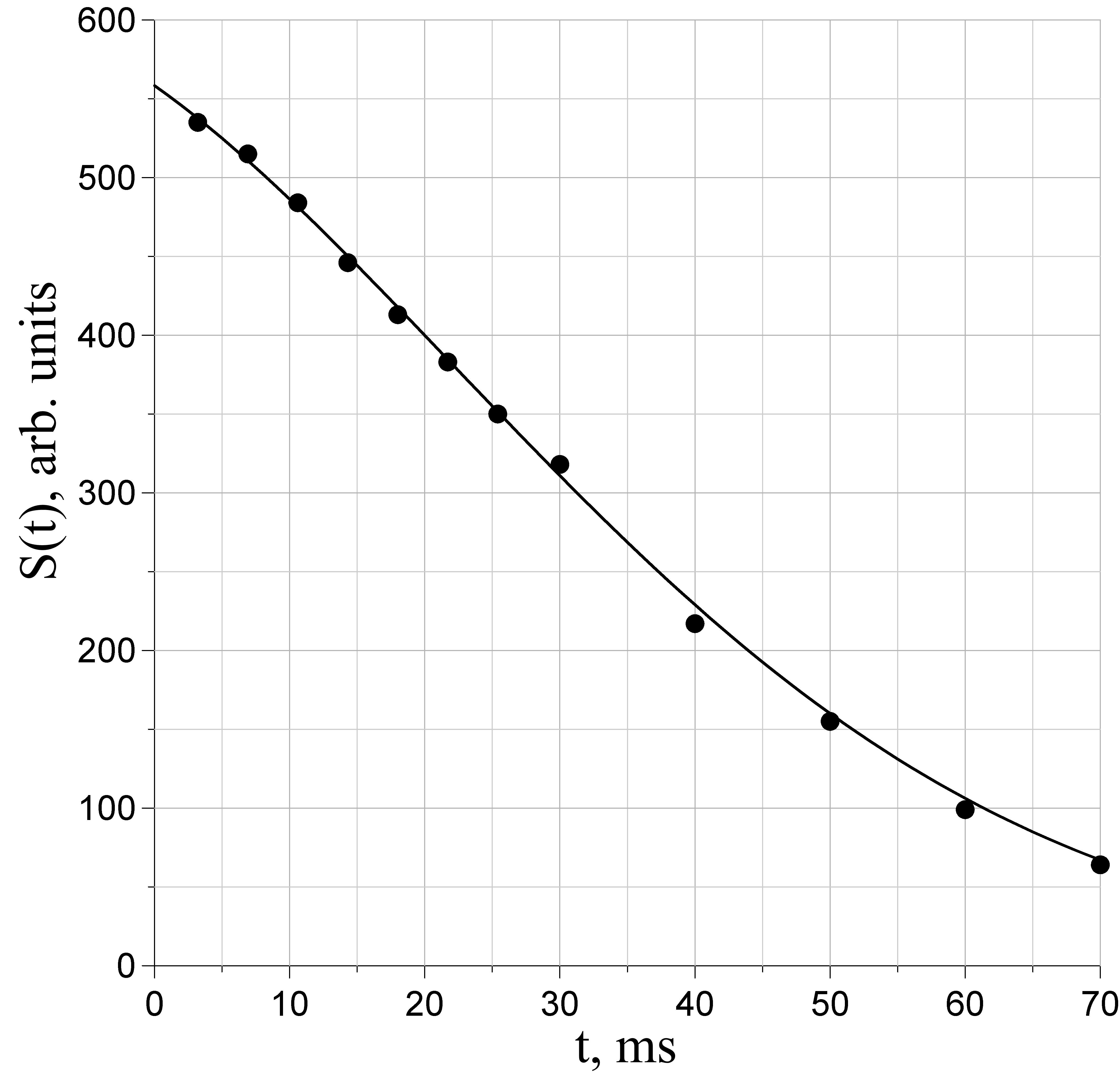
Parameters $$$a$$$ and $$$b$$$ are provided by the multi-point algorithm with clamping (MPC), while $$$w$$$ and $$$\epsilon$$$ are derived from them in order to match the function with the experimental curve. Figure 1 shows an example of the FRA being fitted over an experimental curve.
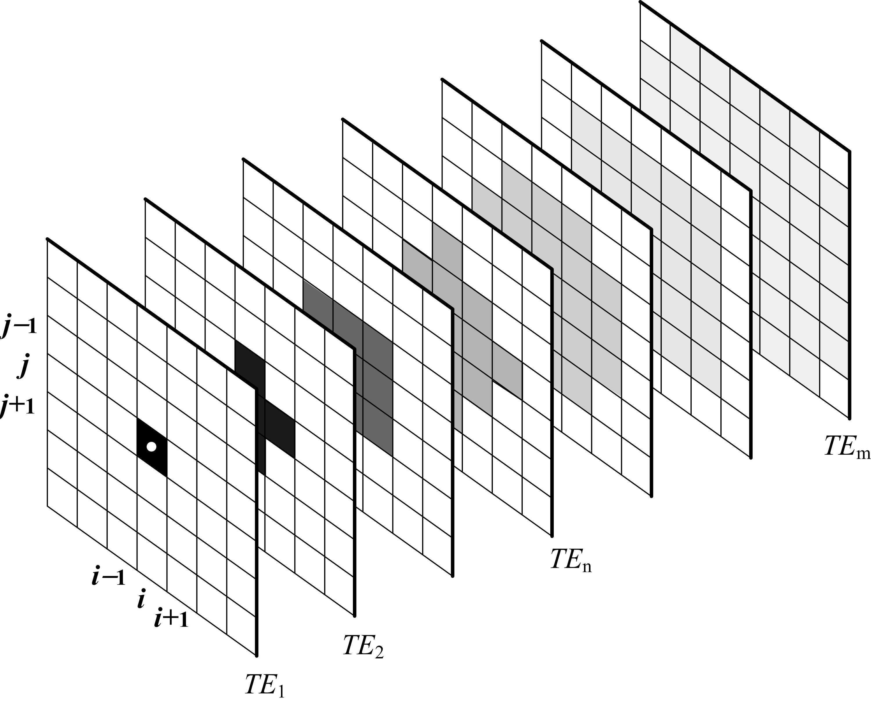
In order to maintain signal-to-noise ratio (SNR), the concept of branching averaging with statistical weighting was introduced (Fig. 2). As the signal amplitude (unlike noise) decays with TE, the loss of SNR is compensated by an increased averaging of neighboring pixels for subsequent TEs. This averaging leads to reduced spatial resolution, and to mitigate this, the number of averaged pixels is set proportional to TE.
The method presented in this article was tested on a number of sequences performed on volunteers. These scans were performed on a Siemens Symphony scanner using an unmodified GRE sequence. Twelve separate echoes were acquired with each sequence, with echo times between 2.6 ms and 70 ms and a TR of 75 ms.
Results
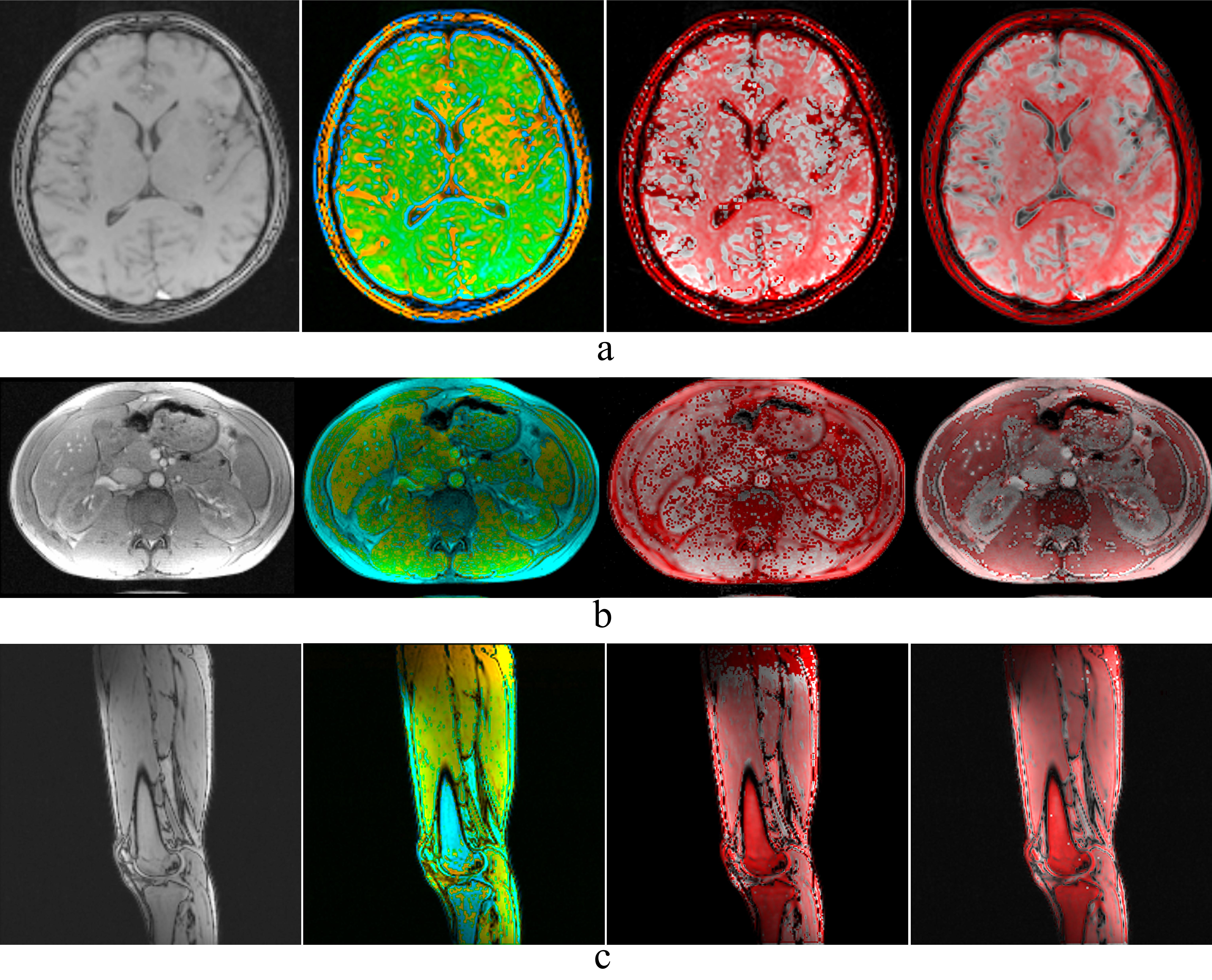
Fig.3 shows the results. The T2 and T0.5 maps are different. For example, the average T2 time of the liver in the abdominal images is 32 ms, while the average T0.5 time is 18 ms. Furthermore, the gradient colormap noticeably highlights the borders between different organs, where changes in susceptibilities between different organs create magnetic field gradients.Discussion and Conclusion
The concept of parameterization splits every original GRE image into a series of maps, showing spatial distribution of parameters like T2, average gradients, T0.5, or others that were previously considered to be impossible to acquire using a GRE sequence. Thus, from pure intensity rendering in conventional GRE imaging, we come to mapping of physical parameters relevant to specific clinical applications, such as BOLD. Many more parameters can be derived from the shape of the relaxation curve, such as total volume under the curve, decay rate and spin density. The concept of parameterization of GRE imaging might improve classification of tissues could potentially help in the detection of tumors.Acknowledgements
No acknowledgement found.References
1. Yablonskiy D.A, Haacke E.M. Theory of NMR signal behavior in magnetically inhomogeneous tissues – the static dephasing regime. Magn Reson Med. 1994;32(6):749–763.
2. Sukstanskii A.L, Yablonskiy D.A. Gaussian approximation in the theory of MR signal formation in the presence of structure-specific magnetic field inhomogeneities. Journal of Magnetic Resonance 2003;163:236–247.
3. Sukstanskii A.L, Yablonskiy D.A. Gaussian approximation in the theory of MR signal formation in the presence of structure-specific magnetic field inhomogeneities. Effects of impermeable susceptibility inclusions. Journal of Magnetic Resonance 2004;167:56-67.
4. Kiselev V.G. Effect of magnetic field gradients induced by microvasculature on NMR measurements of molecular self-diffusion in biological tissues. Journal of Magnetic Resonance 2004;170:228–235.
5. Dickson J.D, Ash T.W.J, Williams G.B, Sukstanskii A.L, Ansorge R.E, Yablonskiy D.A. Quantitative phenomenological model of the BOLD contrast mechanism. Journal of Magnetic Resonance 2011;212:17–25.
6. Knight M.J, Kauppinen R.A. Diffusion-mediated nuclear spin phase decoherence in cylindrically porous materials. Journal of Magnetic Resonance 2016;269:1–12.
7. Wharton S, Bowtell R. Fiber orientation-dependent white matter contrast in gradient echo MRI. Proc Natl Acad Sci USA 2012;109:18559– 18564. Supporting information 10.1073/pnas.1211075109.
8. Fernandez-Seara M.A, Wehrli F.W. Postprocessing technique to correct for background gradients in image-based R2* measurements. Magn Reson Med. 2000;44:358–366.
9. Dahnke H, Schaeffter T. Limits of detection of SPIO at 3.0T using T2* relaxometry. Magn Reson Med 2005;53:1202–1206.
10. Yablonskiy D.A. Quantitation of intrinsic magnetic susceptibility-related effects in a tissue matrix. Phantom study. Magn Reson Med. 1998;39:417–428.
11. Hahn E.L. Spin echoes, Physical Review 1950;80(4):580-594.
Figures