2764
Improved ADC Estimation Technique Using Regularized Nonlinear Least Squares Fitting1Radiology, Mayo Clinic, Rochester, MN, United States
Synopsis
A high-performance model-based regularized non-linear-least-squares ADC fitting technique has been designed and implemented. Phantom testing shows a reduction in noise with significant retention of detail, while providing < 10 sec computation for 3D acquisitions with 4 b-values.
Purpose
Calculations of apparent diffusion coefficients (ADC) from diffusion-weighted imaging (DWI) frequently occur in low-SNR1 environments, and can be
problematic for regions far from receiver coils. ADC calculations are typically performed2 via log-linear-least-squares (LLLS), which can easily fail in
low SNR regions. We present a combination of non-linear-least-squares (NLLS) fit and regularization (Regularized NLLS) for improved stability in a
computationally efficient form for reducing noise in the resulting ADC image. Purpose
Methods
Methods
Three different ADC calculation methods were considered, LLLS, NLLS, and Regularized NLLS. We begin with the DWI signal model, $$$g[n,t]=m[n]e^{-b_t\cdot ADC[n]}$$$, where $$$g[n,t]$$$ is the observed DWI signal at position $$$n$$$ and time $$$t$$$, $$$m[n]$$$ is the signal intensity in the absence of diffusion, $$$b_t$$$ is the b-value applied at time $$$t$$$, and $$$ADC[n]$$$ is the apparent diffusion coefficient at position $$$n$$$. We need to solve for both $$$m[n]$$$ and $$$ADC[n]$$$ given $$$g[n,t]$$$ (DWI images) and $$$b_t$$$. LLLS involves calculating $$$log(g[n,t_b]/g[n,t_0])$$$ at each voxel and solving (through the normal equations) for the slope of this parameter vs. b-value. Variable Projection3 (VARPRO) was utilized for both variants of NLLS models to reduce their dimensionality. VARPRO leverages the facts that the NLLS cost functional is quadratically dependent upon $$$m$$$, and that we can directly calculate $$$\hat{m}$$$, the optimal value of $$$m$$$, for a given $$$ADC$$$ under consideration. This transforms an expensive 2D search over $$$ADC$$$ and $$$m$$$ into a 1D search across $$$ADC$$$, implemented here as a golden section search, while the optimal (least-squares) $$$m$$$ is implicitly calculated at each step.
Our regularized NLLS solver further builds upon this process by adding a regularization term to the minimization problem. In the equations below, we seek to minimize $$$J$$$. The first ($$$\lambda$$$-weighted) summation in (1) provides regularization: $$$D_i$$$, a finite differences operator, where $$$\Omega$$$ is the local neighborhood, promotes local smoothness within the $$$ADC$$$ estimate. The second summation enforces fidelity of the solution to the observed DWI signal, $$$g$$$. The subsequent equations illustrate the VARPRO technique: (2) a new matrix function $$$H_t(ADC)=e^{-b_t\cdot ADC}$$$ is introduced, (3) the least squares solution for $$$\hat{m}$$$ is calculated from $$$g$$$ via the Moore-Penrose pseudoinverse of $$$H$$$, (4) replacement of $$$m$$$ provides the final form with variable projection in place.
\begin{align}J(m,ADC)&=\lambda\sum_{i\in\Omega}\left\Vert{D_i\cdot ADC}\right\Vert^p_p+\sum_t\sum_n\left|{m[n]e^{-b_t\cdot ADC[n]}-g[n,t]}\right|^2&(1)\\&=\lambda\sum_{i\in\Omega}\left\Vert{D_i\cdot ADC}\right\Vert^p_p+\sum_t\left\Vert{H_t(ADC)m-g_t}\right\Vert^2_2&(2)\\\hat{m}&=\left[H(ADC)\right]^+g&(3)\\J(m,ADC)&=\lambda\sum_{i\in\Omega}\left\Vert{D_i\cdot ADC}\right\Vert^p_p+\left\Vert{H(ADC)\left[H(ADC)\right]^+g-g}\right\Vert^2_2&(4)\\\end{align}
To test these algorithms experimentally, we acquired a stack of EPI DWI images of the QIBA4 diffusion phantom (Figure 1) (NEX@b=[1@0, 1@100, 3@600, 9@1000]; directions=[x,y,z]), reconstructed at 256 x 256 x 26, (Figure 2) with a 3.0T GE HD 16.0 MRI system and a production 8-channel head coil (readout SI) with SENSE acceleration factor of 2 (AP). The phantom's ice bath was verified to be at 0°C prior to imaging. DWI reconstruction was performed via GE's Orchestra software, with complex averaging of NEXs and low-frequency phase correction5. The resulting directional images were geometrically averaged to create a set of diffusion weighted images to use as input for ADC calculations.
In our implementation, $$$J$$$ is minimized via sequential binary optimizations ($$$\alpha$$$-expansion), with each binary decision solved via graph cuts6, which were solved efficiently via the GridCut7 implementation. We parallelize (via MPI8 and OpenMP9) outside of the GridCut implementation, allowing all of the processing steps to be performed in parallel across acquired slices. This allows the full 3D DWI source volume with four b-values to be processed (ADC images generated from DWI images) in ~6s on a computing workstation with two Intel Xeon E5-2760v2 (2.6GHz x 10 core/20 thread) processors. For this work, we used 100 $$$\alpha$$$-expansion iterations with fixed-interval continuation, manually selected $$$\lambda$$$, and set $$$p=1.5$$$ to trade off smoothness while minimizing "staircasing10."
Results
Figure 2 shows trimmed slices through the phantom, acquired approximately where indicated in Figure 1. Three vials are visible, with the fourth (0% PVP; water) indistinguishable from the surrounding bath. The improvement in noise behavior and sharpness retention is visible both in the regularized NLLS result, and in the line profiles (bottom). Figure 3 presents statistics from 1000-voxel samples within each of the seven central vials of the QIBA phantom. As expected, there is minimal difference between the techniques in average values (top), while regularized NLLS achieves a significant reduction in the standard deviation (bottom).Discussion
We have designed and implemented a high-performance (<10s per exam) model-based ADC estimation technique providing a regularized non-linear-least-squares fit. We have demonstrated reduced noise within uniform sections of a phantom, with substantial retention of sharpness. Future work will include integration into the overall reconstruction process as well as radiological evaluation of the technique.Acknowledgements
Funding Sources:
DOD W81XWH-15-1-0341
Mayo Clinic Discovery Translation Grant
References
- Mazaheri, Y, Diffusion-weighted MRI of the prostate at 3.0 T: Comparison of endorectal coil (ERC) MRI and phased-array coil (PAC) MRI—The impact of SNR on ADC measurement, European Journal of Radiology, 82(10):e515-520 (2013)
- Jones, DK, Diffusion MRI, Oxford University Press, 2010
- Golub, GH, The differentiation of pseudoinverses and nonlinear least squares problems whose variables separate, SIAM Journal on Numerical Analysis 10(2):413–432 (1973)
- Boss, MA, QIBA Perfusion, Diffusion, & Flow MRI Technical Committee: Current Status, RSNA Poster, 2013
- McKinnon, GC, Phase Corrected Complex Averaging for Diffusion Weighted Spine Imaging, ISMRM 2002, #802
- Kolmogorov, C, What energy functions can be minimized via graph cuts?, IEEE Transactions on Pattern Analysis and Machine Intelligence, 26(2):147-159 (2004)
- Jamriška, O, Cache-efficient graph cuts on structured grids, IEEE Conference on Computer Vision and Pattern Recognition, 16-21 June 2012
- http://www.mpi-forum.org/
- http://www.openmp.org/
- Buades A, The staircasing effect in neighborhood filters and its solution, IEEE Transactions on Image Processing, 15(6):1499-1505 (2006)
Figures
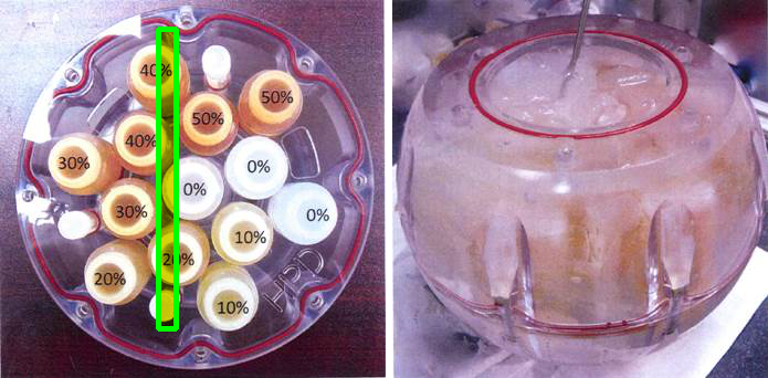
Figure 1:
Left: Photo of QIBA phantom with the approximate location of the slice displayed in Figure 2 highlighted. The central seven vials were used for the statistics in Figure 3.
Right: the phantom as prepared in ice bath prior to imaging.
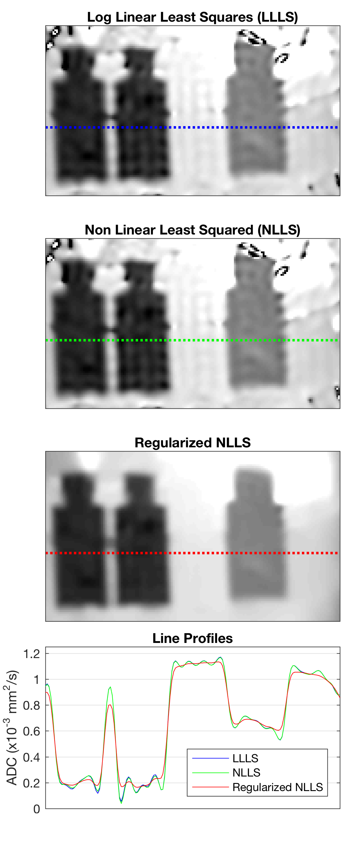
Figure 2:
One slice through the phantom as obtained with the three considered ADC calculation techniques. Visible (L-R) in each are are vials of 40%, 40%, 0%, and 20% PVP. (The 0% PVP (100% water) vial is not distinct from the surrounding water signal.)
Line profiles at the indicated position are shown in the bottom graph. Note the reduction in variation within vials while substantially retaining sharpness.
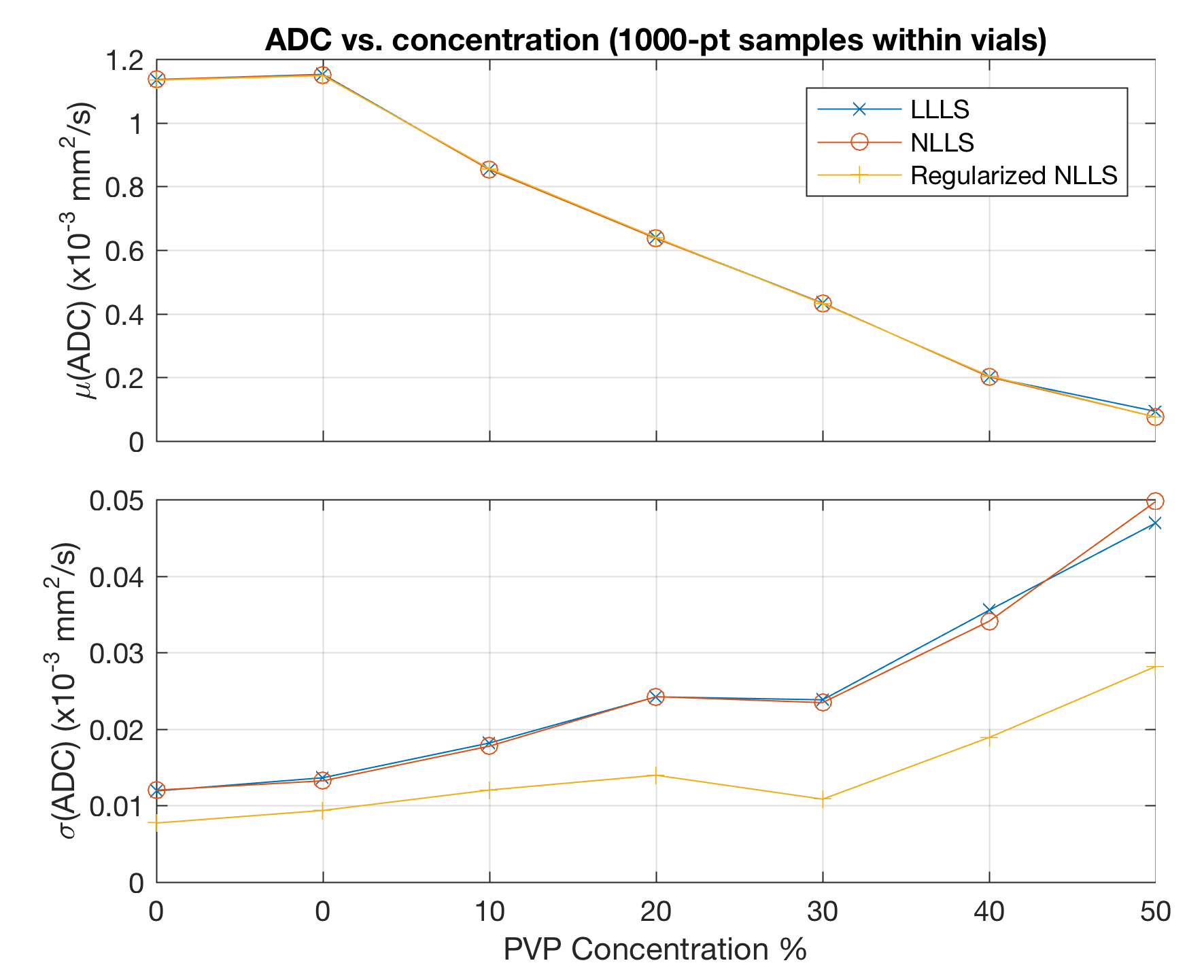
Figure 3:
Mean (top) and standard deviation (bottom) of calculated ADC values within 1000-voxel samples placed in vials of varying PVP concentration. The Regularized NLLS calculation shows reduced standard deviation, as expected.