Introduction

Charcot-Marie-Tooth disease (CMT) diseases are a heterogeneous group of inherited peripheral neuropathies that result in muscle atrophy and impaired sensory function. Recent clinical trials¹ have noted a need for novel biomarkers capable of tracking disease progression in CMT. Recent work from our lab¹ has further indicated that sciatic nerve (SN) hypertrophy is related to the level of impairment in certain CMT subtypes (e.g., CMT1A) and, therefore, may be a viable biomarker in these patients. Currently, segmentation of the SN from MRI images of the thigh requires a labor-intensive process. Furthermore, due to the size and nature of the SN, large inter-rater variabilities are often observed. The goal of this study was to develop an automated method to accurately and consistently segment peripheral nerves. More specifically, we deployed the U-Net convolutional neural network (CNN) architecture², which has been successfully applied to a number of 3D biomedical image segmentation problems³. The architecture consists of two paths: i) an analysis path that downsamples the input volume to capture image features and ii) a symmetric, expanding path that upsamples these feature for localization/segmentation purposes.

Methods

Axial T1-weighted MRI volumes were acquired at 3.0 T (Philips Achieva) in one thigh immediately proximal to the knee. Additional parameters included: PROSET fat suppression, TR/TE=60/11 ms, resolution=0.75x0.75x3 mm (40 slices), matrix=256x256x40, scan time=3 min. Data from 72 subjects (34 CMT, 38 controls) were acquired and regions-of-interest (ROIs) were manually defined for the SN. Our custom implementation of the U-Net architecture was written in Python 2.7 using Keras 2.0 and a Tensorflow backend. Data were first corrected for bias field via ANTS (N4BiasFieldCorrection⁴). To reduce convergence time during training, slices were then cropped at a 48x48 window (36x36 mm) about the SN. The cropped training volumes were fed in user-defined sized batches into the U-Net optimizing validation dice-coefficient. Training was performed on a NVIDIA Titan X GPU via stochastic gradient descent backpropagation with a learning rate/momentum=0.00001/0.99 over 5000 epochs. Four distinct implementations of the U-Net network architecture were tested: 1) a 2D U-Net with data augmentation (via nonlinear elastic transforms to minimize overfitting), 2) a 3D U-Net with data augmentation, 3) a 3D U-Net with data augmentation and batch normalization (minimizes internal covariance shift⁵) and 4) a 3D U-Net without data augmentation or batch normalization. Three trials were conducted for each of the 4 networks, each with random partitions of subject data into training (64% of subjects), validation (16%), and testing (20%) datasets. This data analysis pipeline is summarized in Fig. 1.

Results

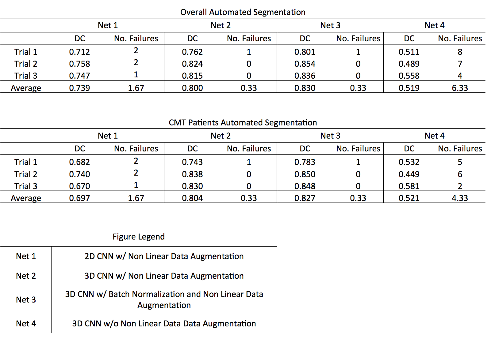
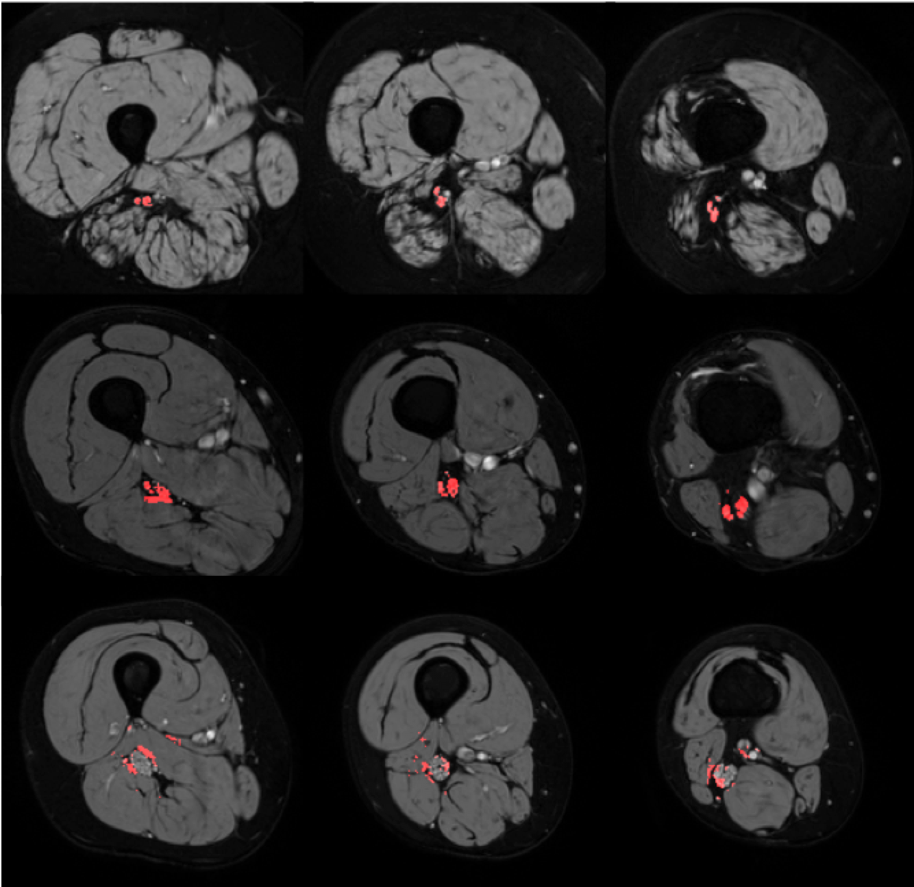
Results from the three trials are shown in Fig. 2. Failed segmentations were defined as segmentations yielding dice coefficients < 0.5. This distinction for successful segmentations was necessitated by the occasional misclassification (shown in the bottom row of Fig. 3), which was most often observed in patients with CMT and points to the need for larger datasets to minimize overfitting during network training. Removing these failed segmentations, we report the mean performance of each network across the three trials in Fig. 2. All three networks utilizing on-the-fly elastic transformations outperformed the 3D CNN trained on unaugmented data, while the 3D CNN trained on augmented data outperformed the 2D CNN trained on augmented data. The top network performance from was the batch normalizing 3D CNN, only failing to successfully segment a single CMT or control MRI volume out of all three trials.

Discussion and Conclusions

These results demonstrate the advantage of utilizing 3D convolutional filters, which fully capture the structural nature of the sciatic nerve, over 2D filters. The improved dice-coefficient in networks employing on-the-fly non-linear elastic deformations also demonstrates the necessity for generating unseen, but structurally similar, MR images while training the network to prevent overfitting. This is especially critical in biomedical applications, given the limited availability of large, expertly labeled datasets. Together, these findings demonstrate that CNNs are capable of producing robust, high-quality segmentations in small structures such as the sciatic nerve. By removing the need for expertly trained raters, CNNs may allow for a more consistent estimation of sciatic nerve diameters. Future work includes: 1) estimating the relationship between CNN-derived sciatic nerve diameters and disability and 2) applying this pipeline in other nerves (e.g. the median nerve).

Acknowledgements

We thank NIH K25 EB013659 and R01 NS97821 for funding.